Comparing compensation – No. 2 The application of the equal line method
Cat. No.: HR4-104/2-2023E-PDF
ISBN: 978-0-660-49637-5
Table of Contents
- 1. Purpose
- 2. Introduction to the equal line method
- 3. Rules for using the equal line method
- 4. Calculating the increase in compensation using the factor
- 5. Detailed example using the equal line method
- 5.1. Step 1: Create two regression lines by plotting the data on a graph
- 5.2. Step 2: Identify female job classes falling below the male regression line
- 5.3. Step 3: Determine the equation of the male regression line
- 5.4. Step 4: Recalculate total hourly compensation for male job classes using the equation of the male regression line and the job values of comparable female job classes
- 5.5. Step 5: Calculate the factor
- 5.6. Step 6: Determine the increase in compensation
- 5.7. Step 7: Graph predominantly male and female job class data after pay equity adjustment
- 6. Referenced Pay Equity Act provisions
- 7. Referenced Pay Equity Regulations
1. Purpose
This Interpretation, Policy and Guideline (IPG) provides guidance on the application of the equal line method prescribed in section 50 of the Pay Equity Act and section 12 of the Pay Equity Regulations:
- Section 2: Introduction to the equal line method.
- Section 3: Rules for using the equal line method.
- Section 4: Calculating the increase in compensation using the factor.
- Section 5: Detailed example using the equal line method.
Note: For all mentions of total compensation, this refers to the total hourly compensation before pay equity. Also, all mentions of female job classes and male job classes refer to predominantly female job classes and predominantly male job classes, respectively.
This IPG is the second in a series that addresses the comparison of compensation. The other IPGs in this series are:
- No. 1: The Application of the Equal Average Method.
- No. 3: What to Do When the Regression Lines Cross: The Modified Version of the Equal Line Method.
- No. 4: What to Do When the Regression Lines Cross: The Equal Average, Segmented Line and Sum of Differences Methods.
- No. 5: Guidance on the Use of Other Methods to Compare Compensation.
This document does not replace expert legal and/or compensation advice. This document is technical in nature and should not be used as a plain language resource. Plain language resources are available at https://www.payequitychrc.ca/en.
The term employer in this document can also refer to a group of employers that has been recognized by the Pay Equity Commissioner.i
A note on data validation and verification
The collection or use of incorrect or inaccurate data can have a negative impact on organizations. This is especially true when dealing with employee pay equity data (e.g., data used to determine job classes, gender predominance, total hourly compensation, job values, etc.). For example, when using a pay equity method for the comparison of compensation, inaccurate data can create extreme pay differences within similar job classes.
Since these methods are used to make pay adjustments, data validation and verification procedures for employee data should be a priority. Instances of large disparities of compensation within pay bands, for example, can produce unclear or confusing results. Should situations of this nature occur, they should be investigated and scrutinized before proceeding with the use of any pay equity method.
When comparing compensation for pay equity and performing calculations, it is a best practice to use numbers with four or five decimal places and then round to two decimal places at the end. If rounding is done before, it increases the risk of carrying through calculation errors, which may have an impact on your final results and the determination of whether a specific method has worked.
2. Introduction to the equal line method
Under the Pay Equity Act (the Act), an employer or pay equity committee must compare the total compensation of predominantly female job classes with the total compensation of predominantly male job classes of equal value to determine whether there are differences in compensation.ii The employer or pay equity committee is required to do this to identify and address any pay equity gaps in the workplace.
The Act prescribes two methods that employers and pay equity committees can use to compare total compensation: the equal average method and the equal line method.iii
The equal line method uses regression lines to compare the total compensation of female and male job classes. The equal line method can be used only with data sets that can be approximated using linear regression.
For information on the equal average method, see Comparing Compensation – No. 1: The Application of the Equal Average Method.
3. Rules for using the equal line method
An employer or pay equity committee that chooses to use the equal line method to compare the compensation of predominantly female job classes with the compensation of predominantly male job classes must follow the rules prescribed by the Pay Equity Act:
- Two regression lines must be created: one for female job classes and one for male job classes.iv Each regression line represents the relationship between the value of work and total hourly compensation.
- The compensation associated with a female job class is to be increased if:
- The female regression line is entirely below the male regression line, as shown in the figure below; and,
-
The female job class is below the male regression line, as shown in the figure below for job classes f1, f2, f3, f4, f5, f8, f9, f11 and f12.v
- The increase owed is determined by multiplying a factor by the difference between the compensation associated with the female job class and the compensation associated with a male job class with an equal job value, were such a job class located on the male regression line.vi
-
After increases in compensation are made for female job classes, the female regression line must coincide with the male regression line, as shown in the figure below.vii
For what to do when the regression lines cross, see Comparing Compensation – No. 3: What to Do When the Regression Lines Cross: The Modified Version of the Equal Line Method.
4. Calculating the increase in compensation using the factor
Any increases in compensation owed to predominantly female job classes must be made in such a way that, after the increase, the female and male regression lines coincide.
This is accomplished by multiplying the differences in compensation between male and female job classes by a factor that is determined using the following formula:viii
Factor = [(A × B) ÷ C] + [D − (E × B)]
The factor will have a value between 0 and 1.ix
The formula is further explained in Section 5 of this document through an example.
5. Detailed example using the equal line method
The following example provides step-by-step guidance on how to use the equal line method.
For this example, Company B’s pay equity committee has calculated the total compensation for each predominantly female and predominantly male job class. To compare total compensation, the committee decides to use the equal line method.
The pay equity plan includes 12 male job classes and 12 female job classes.
Table 1 provides the job value and total hourly compensation for each job class.
Table 1: Company B job classes, job values and total hourly compensation
Male job classes
| Job class | Job value | Total hourly compensation |
|---|---|---|
| m1 | 50 | $23.00 |
| m2 | 100 | $20.00 |
| m3 | 125 | $24.00 |
| m4 | 150 | $31.00 |
| m5 | 200 | $27.00 |
| m6 | 225 | $33.00 |
| m7 | 250 | $31.00 |
| m8 | 300 | $35.00 |
| m9 | 350 | $44.00 |
| m10 | 400 | $45.00 |
| m11 | 450 | $46.00 |
| m12 | 500 | $56.00 |
Female job classes
| Job class | Job value | Total hourly compensation |
|---|---|---|
| f1 | 50 | $15.00 |
| f2 | 70 | $17.00 |
| f3 | 85 | $15.00 |
| f4 | 115 | $21.00 |
| f5 | 145 | $18.00 |
| f6 | 160 | $30.00 |
| f7 | 180 | $35.00 |
| f8 | 275 | $31.00 |
| f9 | 305 | $37.00 |
| f10 | 360 | $47.00 |
| f11 | 415 | $45.00 |
| f12 | 525 | $46.00 |
5.1. Step 1: Create two regression lines by plotting the data on a graph
As a first step to using the equal line method, the pay equity committee must create regression lines by plotting the data on a graph.
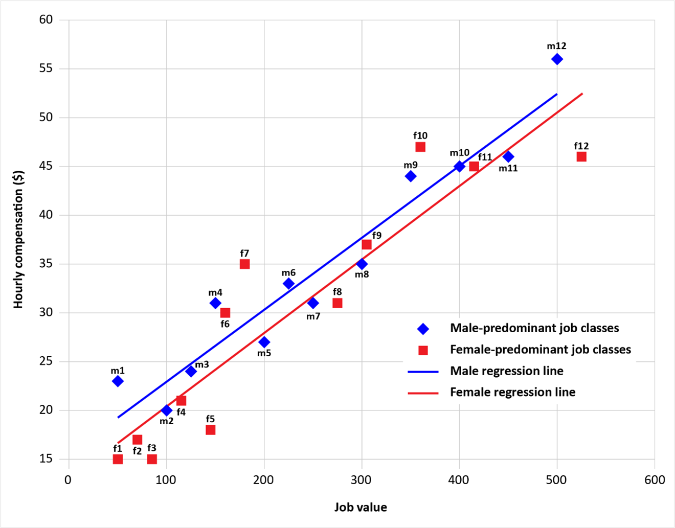
Using the data from Table 1, the pay equity committee plots total hourly compensation on the y-axis and job values on the x-axis. They plot the amounts for female and male job classes separately.
Female job classes are represented by red squares, and male job classes are represented by blue diamonds.
Two regression lines are created, estimating total hourly compensation for male and female job classes, respectively.
Figure 1: Job values and total hourly compensation for Company B job classes, with male and female regression lines
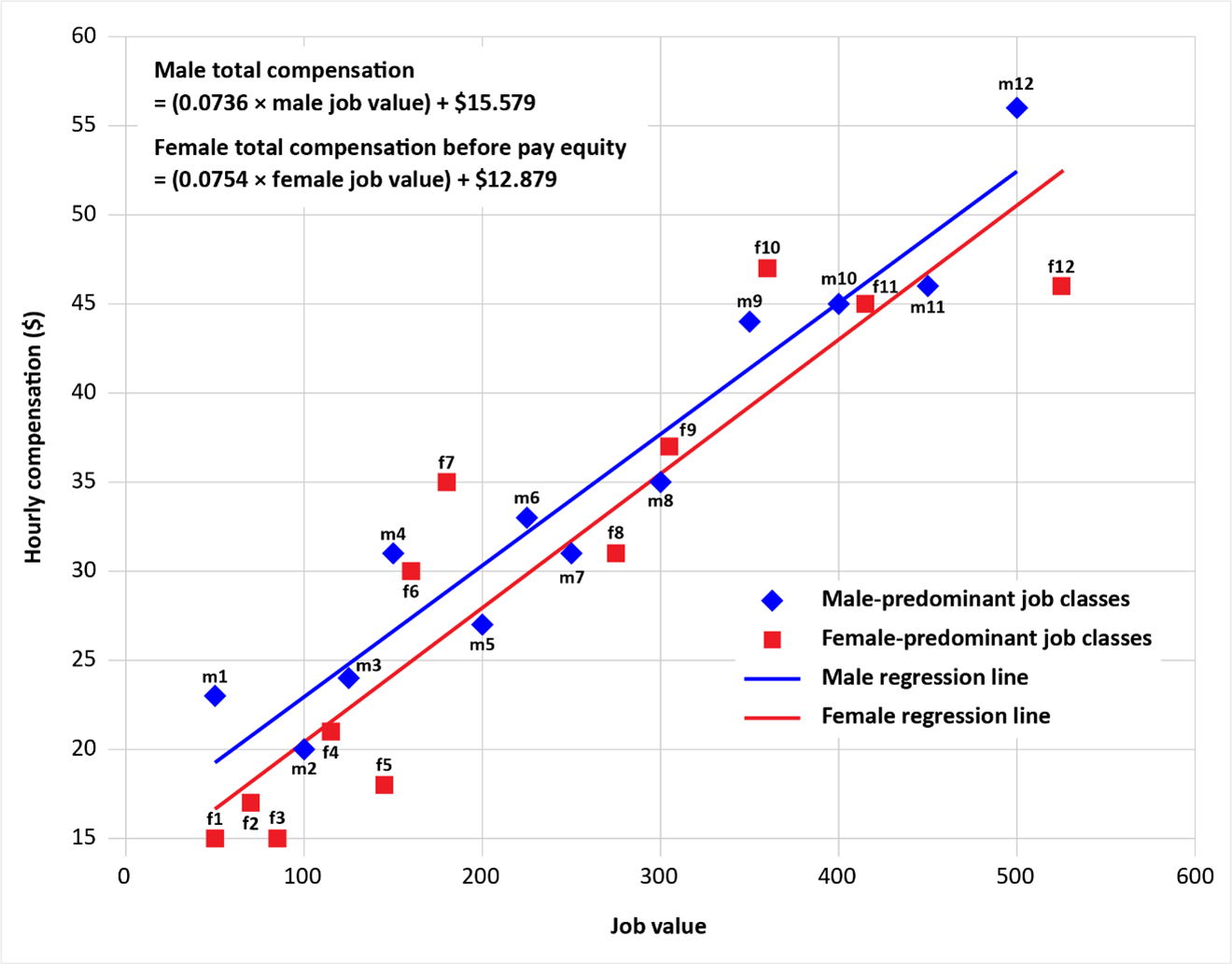
The blue regression line in Figure 1 represents the estimated male total compensation, based on the male job values. Its formula, Equation 1, is as follows:
Male total compensation = (slope × male job value) + y-intercept
Male total compensation = (0.0736 × male job value) + $15.579
More information on creating a regression line is provided in Section 5.3.
The regression lines don’t cross within the relevant range of job values. Therefore, the pay equity committee can use the equal line method as outlined in section 50 of the Pay Equity Act (the Act).
For what to do when the regression lines cross, see Comparing Compensation – No. 3: What to Do When the Regression Lines Cross: The Modified Version of the Equal Line Method.
5.2. Step 2: Identify female job classes falling below the male regression line
Once the pay equity committee creates the male and female regression lines, they note that:
- The female regression line is entirely below the male regression linex; and,
- Some female job classes are below the male regression line.xi
As per the Act, if these two criteria are met, female job classes that are below the male regression line are owed an increase in compensation. These are identified as eligible female job classes.
As shown in Figure 1, the following female job classes are below the male regression line and are owed an increase in compensation: f1, f2, f3, f4, f5, f8, f9, f11 and f12. The following female job classes are above the male regression line and are not owed an increase in compensation: f6, f7 and f10.
5.3. Step 3: Determine the equation of the male regression line
Some female job classes in the pay equity plan are owed an increase in compensation. The increase in compensation for each of these job classes must be determined by multiplying the factor by an amount equal to the difference between the compensation associated with the female job class and the compensation associated with a male job class with an equal job value, were such a job class located on the male regression line.xii
To begin, the pay equity committee must calculate the difference between the compensation associated with each female job class and the compensation associated with a male job class with an equal job value, were such a job class located on the male regression line. To do this, the pay equity committee must determine the equation of the male regression line for the purpose of estimating total hourly compensation.
In this example, the equation of the male regression line is given by Equation 1:
Male total compensation = (0.0736 × male job value) + $15.579
Male total compensation is the total hourly compensation associated with each male job class. The slope of the regression line is 0.0736. Male job value is the job value associated with each male job class. The y-intercept of the regression line is $15.579.
Note: The equation for a regression line can be determined using graphing software such as Excel or a statistical software package such as R, SAS or SPSS. To determine the equation of the male regression line in Excel, start by right-clicking the plotted points for the male job classes and selecting “Add trend line.” Once the trend line is visible, right-click it and select “Display equation on chart.” Once the equation is displayed, it can be used to calculate the estimated compensation an employee in a male job class would be paid given different job values.
5.4. Step 4: Recalculate total hourly compensation for male job classes using the equation of the male regression line and the job values of comparable female job classes
Using the data from Table 1, Company B’s pay equity committee uses the equation of the male regression line to recalculate the total hourly compensation of male job classes using job values equal to those of comparable female job classes.
This step ensures that the pay equity committee is comparing female job classes with male job classes of equal value. The pay equity committee uses the equation of the male regression line to recalculate the total hourly compensation for male job classes of equal value to their female counterparts. This step is required so that female job classes can be compared to male job classes of the same job value.
Table 2 below provides the adjusted male total hourly compensation estimates using Equation 1, the equation of the male regression line, calculated in Step 3 above.
For example, the adjusted total hourly compensation for m1 in Table 2 is calculated as follows:
m1 adjusted total hourly compensation = (0.0736 × male job value) + $15.579
= (0.0736 × 50) + $15.579
= $19.26
The new m1 total hourly compensation, calculated using Equation 1, is $19.26.
For example, the adjusted total hourly compensation for m2 in Table 2 is calculated as follows:
m2 adjusted total hourly compensation = (0.0736 × male job value) + $15.579
= (0.0736 × 70) + $15.579
= $20.73
The new m2 total hourly compensation, calculated using Equation 1, is $20.73.
Table 2 also demonstrates that the job values of the male job classes are the same as those of the female job classes.
Company B’s pay equity committee uses the new male total hourly compensation amounts for the remaining calculations to determine the increases owed to eligible female job classes. The amounts in Table 1 are no longer relevant.
Table 2: Company B job classes, job values and total hourly compensation, with male job values equal to job values of comparable female job classes and male total hourly compensation adjusted using Equation 1
Male job classes
| Job class | New job value* | New total hourly compensation** |
|---|---|---|
| m1 | 50 | $19.26 |
| m2 | 70 | $20.73 |
| m3 | 85 | $21.84 |
| m4 | 115 | $24.04 |
| m5 | 145 | $26.25 |
| m6 | 160 | $27.36 |
| m7 | 180 | $28.83 |
| m8 | 275 | $35.82 |
| m9 | 305 | $38.03 |
| m10 | 360 | $42.08 |
| m11 | 415 | $46.12 |
| m12 | 525 | $54.22 |
| * New male job values are equal to the job values of comparable female job classes. | ||
| ** New male total hourly compensation amounts are estimated using Equation 1. | ||
Female job classes
| Job class | Job value | Total hourly compensation |
|---|---|---|
| f1 | 50 | $15.00 |
| f2 | 70 | $17.00 |
| f3 | 85 | $15.00 |
| f4 | 115 | $21.00 |
| f5 | 145 | $18.00 |
| f6 | 160 | $30.00 |
| f7 | 180 | $35.00 |
| f8 | 275 | $31.00 |
| f9 | 305 | $37.00 |
| f10 | 360 | $47.00 |
| f11 | 415 | $45.00 |
| f12 | 525 | $46.00 |
5.5. Step 5: Calculate the factor
Now that Company B’s pay equity committee has estimated the new male total hourly compensation amounts outlined in Table 2, they must calculate the factor for each of the female job classes that are owed an increase in compensation.
For this example, detailed calculations will be provided for the first female job class, f1.
The factor is calculated using the following formula:
Factor = [(A × B) ÷ C] + [D − (E × B)]

In this formula:
A is determined by the formula A = F ÷ G, where:
F is the absolute value of the difference between the compensation associated with the predominantly female job class and the compensation associated with a predominantly male job class, were such a job class located on the male regression line, in which the value of the work performed is equal to that of the predominantly female job class.
G is the compensation associated with such a predominantly male job class.
In this example, F is the absolute value, expressed as ABS(Number), or the positive value resulting from the difference between the hourly compensation associated with the predominantly female job class and the hourly compensation associated with a predominantly male job class of equal value, were it located on the male regression line.
For female job class f1, A is calculated as follows:
A = F ÷ G
= [ABS (f1 compensation − m1 compensation)] ÷ m1 compensation
= [ABS ($15.00 − $19.26)] ÷ $19.26
= $4.26 ÷ $19.26
= 0.2211
The value to use for A in the factor calculation is 0.2211.
B is determined by the formula B = [(H − I) − (J × K)] ÷ [L − (M × K)], where:
H is the sum of the products of the job value of each predominantly female job class multiplied by the hourly compensation associated with a predominantly male job class of equal value, were it located on the male regression line.
H = (f1 job value × m1 compensation) + (f2 job value × m2 compensation)
+ (f3 job value × m3 compensation) + (f4 job value × m4 compensation)
+ (f5 job value × m5 compensation) + (f6 job value × m6 compensation)
+ (f7 job value × m7 compensation) + (f8 job value × m8 compensation)
+ (f9 job value × m9 compensation) + (f10 job value × m10 compensation)
+ (f11 job value × m11 compensation) + (f12 job value × m12 compensation)
= (50 × $19.26) + (70 × $20.73) + (85 × $21.84) + (115 × $24.04)
+ (145 × $26.25) + (160 × $27.36) + (180 × $28.83) + (275 × $35.82)
+ (305 × $38.03) + (360 × $42.08) + (415 × $46.12) + (525 × $54.22)
= $104,608.58
I is the sum of products of the job value for each predominantly female job class and the hourly compensation associated with that job class.
I = (f1 job value × f1 compensation) + (f2 job value × f2 compensation)
+ (f3 job value × f3 compensation) + (f4 job value × f4 compensation)
+ (f5 job value × f5 compensation) + (f6 job value × f6 compensation)
+ (f7 job value × f7 compensation) + (f8 job value × f8 compensation)
+ (f9 job value × f9 compensation) + (f10 job value × f10 compensation)
+ (f11 job value × f11 compensation) + (f12 job value × f12 compensation)
= (50 × $15.00) + (70 × $17.00) + (85 × $15.00) + (115 × $21.00)
+ (145 × $18.00) + (160 × $30.00) + (180 × $35.00) + (275 × $31.00)
+ (305 × $37.00) + (360 × $47.00) + (415 × $45.00) + (525 × $46.00)
= $98,895.00
J is determined by the formula J = (P − Q) ÷ R, where:
P is the total of the compensation of all predominantly male job classes, were such job classes located on the male regression line, in which the value of the work performed is equal to that of the predominantly female job classes.
P = m1 compensation + m2 compensation + m3 compensation + m4 compensation
+ m5 compensation + m6 compensation + m7 compensation + m8 compensation
+ m9 compensation + m10 compensation + m11 compensation + m12 compensation
= $19.26 + $20.73 + $21.84 + $24.04 + $26.25 + $27.36
+ $28.83 + $35.82 + $38.03 + $42.08 + $46.12 + $54.22
= $384.56
Q is the total of the compensation of all predominantly female job classes.
Q = f1 compensation + f2 compensation + f3 compensation + f4 compensation
+ f5 compensation + f6 compensation + f7 compensation + f8 compensation
+ f9 compensation + f10 compensation + f11 compensation + f12 compensation
= $15.00 + $17.00 + $15.00 + $21.00 + $18.00 + $30.00
+ $35.00 + $31.00 + $37.00 + $47.00 + $45.00 + $46.00
= $357.00
R is the sum of the absolute value of the differences, for each eligible predominantly female job class (falling below the male regression line), between the hourly compensation associated with the job class and the hourly compensation associated with a predominantly male job class of equal value, were it located on the male regression line.
R = [ABS (f1 compensation − m1 compensation)] + [ABS (f2 compensation − m2 compensation)] + [ABS (f3 compensation − m3 compensation)] + [ABS (f4 compensation − m4 compensation)]
+ [ABS (f5 compensation − m5 compensation)] + [ABS (f8 compensation − m8 compensation)]
+ [ABS (f9 compensation − m9 compensation)] + [ABS (f11 compensation − m11 compensation)]
+ [ABS (f12 compensation − m12 compensation)]
= [ABS ($15.00 − $19.26)] + [ABS ($17.00 − $20.73)]
+ [ABS ($15.00 − $21.84)] + [ABS ($21.00 − $24.04)]
+ [ABS ($18.00 − $26.25)] + [ABS ($31.00 − $35.82)]
+ [ABS ($37.00 − $38.03)] + [ABS ($45.00 − $46.12)]
+ [ABS ($46.00 − $54.22)]
= $41.31
To calculate J:
J = (P − Q) ÷ R
= ($384.56 − $357.00) ÷ $41.31
= 0.6673
K is the sum of the products of the job value of each eligible predominantly female job class multiplied by the absolute value of the difference between its associated hourly compensation and the hourly compensation associated with a predominantly male job class of equal value, were it located on the male regression line.
K = [f1 job value × ABS (f1 compensation − m1 compensation)]
+ [f2 job value × ABS (f2 compensation − m2 compensation)]
+ [f3 job value × ABS (f3 compensation − m3 compensation)]
+ [f4 job value × ABS (f4 compensation − m4 compensation)]
+ [f5 job value × ABS (f5 compensation − m5 compensation)]
+ [f8 job value × ABS (f8 compensation − m8 compensation)]
+ [f9 job value × ABS (f9 compensation − m9 compensation)]
+ [f11 job value × ABS (f11 compensation − m11 compensation)]
+ [f12 job value × ABS (f12 compensation − m12 compensation)]
= [50 × ABS ($15.00 − $19.26)] + [70 × ABS ($17.00 − $20.73)]
+ [85 × ABS ($15.00 − $21.84)] + [115 × ABS ($21.00 − $24.04)]
+ [145 × ABS ($18.00 − $26.25)] + [275 × ABS ($31.00 − $35.82)]
+ [305 × ABS ($37.00 − $38.03)] + [415 × ABS ($45.00 − $46.12)]
+ [525 × ABS ($46.00 − $54.22)]
= $9,020.92
L is the sum of the products of the job value of each eligible predominantly female job class multiplied by the number calculated for that job class using the equation for A.
L = (f1 job value × A for f1) + (f2 job value × A for f2) + (f3 job value × A for f3)
+ (f4 job value × A for f4) + (f5 job value × A for f5) + (f8 job value × A for f8)
+ (f9 job value × A for f9) + (f11 job value × A for f11) + (f12 job value × A for f12)
= (50 × 0.2211) + (70 × 0.1800) + (85 × 0.3130) + (115 × 0.1266) + (145 × 0.3143) + (275 × 0.1345)
+ (305 × 0.0270) + (415 × 0.0243) + (525 × 0.1516)
= 245.316
The calculation for A for all predominantly female job classes is determined using the formula Ai = Fi ÷ Gi, where i represents the predominantly female job class.
The calculation for A for female job class f1 is provided above.
M is determined by the formula M = N ÷ O, where:
N is the sum of the quotients calculated using the formula set out in A (i.e., A = F ÷ G) in this document, for each eligible predominantly female job class.
N = A for f1 + A for f2 + A for f3 + A for f4 + A for f5 + A for f8 + A for f9 + A for f11 + A for f12
= 0.2211 + 0.1800 + 0.3130 + 0.1266 + 0.3143 + 0.1345 + 0.0270 + 0.0243 + 0.1516
= 1.4924
O is the sum of the absolute values of the differences between the compensation associated with each eligible predominantly female job class and the compensation associated with a predominantly male job class of equal value, were it on the male regression line.
O = ABS (f1 compensation − m1 compensation) + ABS (f2 compensation − m2 compensation)
+ ABS (f3 compensation − m3 compensation) + ABS (f4 compensation − m4 compensation)
+ ABS (f5 compensation − m5 compensation) + ABS (f8 compensation − m8 compensation)
+ ABS (f9 compensation − m9 compensation) + ABS (f11 compensation − m11 compensation)
+ ABS (f12 compensation − m12 compensation)
= ABS ($15.00 − $19.26) + ABS ($17.00 − $20.73)
+ ABS ($15.00 − $21.84) + ABS ($21.00 − $24.04)
+ ABS ($18.00 − $26.25) + ABS ($31.00 − $35.82)
+ ABS ($37.00 − $38.03) + ABS ($45.00 − $46.12)
+ ABS ($46.00 − $54.22)
= $41.31
To calculate M:
M = N ÷ O = 1.4924 ÷ 41.31 = 0.036132
Therefore, to calculate B:
B = [(H − I) − (J × K)] ÷ [L − (M × K)]
= [($104,608.58 − $98,895.00) − (0.667296 × $9,020.9150)]
÷ [(245.316478 − (0.036132 × $9,020.9150)]
= ($5,713.5750 − $6,019.6214) ÷ (245.316478 − 325.943701)
= −306.0464 ÷ −80.6272
= 3.7958
The value to use for B in the factor calculation is 3.7958.
C is calculated as follows:
C is the absolute value of the difference between the hourly compensation associated with the predominantly female job class and the hourly compensation associated with a predominantly male job class of equal value, were it on the male regression line.
C = ABS (f1 compensation − m1 compensation)
= ABS ($15.00 − $19.26)
= $4.26
The value to use for C in the factor calculation is 4.26.
D is calculated as follows:
D is the same value calculated for J.
D = J = 0.667296
The value to use for D in the factor calculation is 0.667296.
E is calculated as follows:
E is the same value calculated for M.
E = M = 0.036132
The value to use for E in the factor calculation is 0.036132.
The final calculation of the factor for female job class f1 is as follows:
Factor = [(A × B) ÷ C] + [(D − (E × B)
= [(0.2211 × 3.7958) ÷ 4.26] + [(0.667296 − (0.036132 × 3.7958)
= 0.197007 + 0.530146
= 0.7272
The final factor calculation amount is 0.7272.
5.6. Step 6: Determine the increase in compensation
The pay equity committee calculates that the factor for female job class f1 is 0.7272.
Increases in compensations for eligible female job classes are calculated by multiplying the difference between the female job class and the hourly compensation associated with a male job by the factor associated with that job class.
The increase in compensation for an eligible female job class is calculated using the following formula:
Increase in compensation = C × factor
For female job class f1, the increase in compensation is calculated as follows:
Increase in compensation for job class f1 = C for f1 × factor for f1
= $4.26 × 0.7272
= $3.10
The increase in total hourly compensation for female job class f1 is $3.10.
The total hourly compensation after pay equity for female job class f1 then becomes
$15.00 + $3.10 = $18.10.
Increases in compensation for all female job classes calculated by the pay equity committee are provided in Table 3.
Table 3: Increases in compensation after pay equity
| Female job class | Total hourly compensation before pay equity | A × B ÷ C | D − (E × B) | C | Factor | Increase in total hourly compensation (C × factor) | Total hourly compensation after pay equity |
|---|---|---|---|---|---|---|---|
| f1 | $15.00 | 0.1971 | 0.5301 | $4.26 | 0.7272 | $3.10 | $18.10 |
| f2 | $17.00 | 0.1831 | 0.5301 | $3.73 | 0.7132 | $2.66 | $19.66 |
| f3 | $15.00 | 0.1738 | 0.5301 | $6.84 | 0.7040 | $4.81 | $19.81 |
| f4 | $21.00 | 0.1579 | 0.5301 | $3.04 | 0.6880 | $2.09 | $23.09 |
| f5 | $18.00 | 0.1446 | 0.5301 | $8.25 | 0.6747 | $5.57 | $23.57 |
| f6 | $30.00 | 0.1388 | 0.5301 | n/a | 0.0000 | $0.00 | $30.00 |
| f7 | $35.00 | 0.1317 | 0.5301 | n/a | 0.0000 | $0.00 | $35.00 |
| f8 | $31.00 | 0.1060 | 0.5301 | $4.82 | 0.6361 | $3.07 | $34.07 |
| f9 | $37.00 | 0.0998 | 0.5301 | $1.03 | 0.6300 | $0.65 | $37.65 |
| f10 | $47.00 | 0.0902 | 0.5301 | n/a | 0.0000 | $0.00 | $47.00 |
| f11 | $45.00 | 0.0823 | 0.5301 | $1.12 | 0.6124 | $0.69 | $45.69 |
| f12 | $46.00 | 0.0700 | 0.5301 | $8.22 | 0.6002 | $4.93 | $50.93 |
5.7. Step 7: Graph predominantly male and female job class data after pay equity adjustment
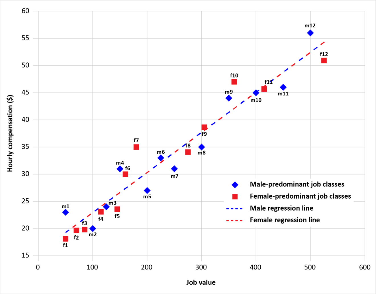
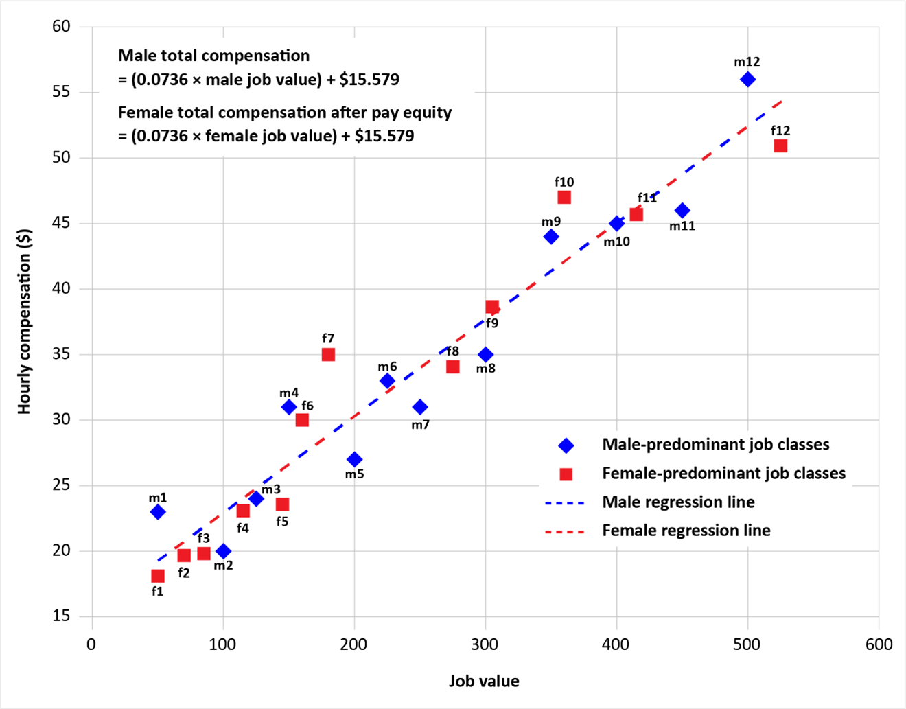
As a final step, the pay equity committee must create a new graph to verify that the increases in compensation associated with eligible female job classes have been calculated in such a way that, after the increases, the female regression line coincides with the male regression line.xiii
The pay equity committee graphs the new total compensation amounts for female job classes after pay equity using the data from Table 3 and the total compensation amounts for male job classes using the data from Table 1. Figure 2 shows the new graph. The female and male regression lines now coincide.
Figure 2: Job values and total hourly compensation for Company B job classes after pay equity adjustment
6. Referenced Pay Equity Act provisions
Group of Employers
4 (1) Two or more employers described in any of paragraphs 3(2)(e) to (i) that are subject to this Act may form a group and apply to the Pay Equity Commissioner to have the group of employers recognized as a single employer.
Comparison
47 An employer — or, if a pay equity committee has been established, that committee — that has calculated under section 44 the compensation associated with each job class must, using the compensation so calculated, compare, in accordance with sections 48 to 50, the compensation associated with the predominantly female job classes with the compensation associated with the predominantly male job classes, for the purpose of determining whether there is any difference in compensation between those job classes.
Compensation comparison methods
48 (1) The comparison of compensation must be made in accordance with the equal average method set out in section 49 or the equal line method set out in section 50.
Equal line method
50 (1) An employer or pay equity committee, as the case may be, that uses the equal line method of comparison of compensation must apply the following rules:
(a) a female regression line must be established for the predominantly female job classes and a male regression line must be established for the predominantly male job classes;
(b) the compensation associated with a predominantly female job class is to be increased only if
(i) the female regression line is entirely below the male regression line, and
(ii) the predominantly female job class is located below the male regression line;
(c) if the compensation associated with a predominantly female job class is to be increased, the increase is to be determined by multiplying the factor calculated in accordance with the regulations by an amount equal to the difference between the compensation associated with the predominantly female job class and the compensation associated with a predominantly male job class, were such a job class located on the male regression line, in which the value of the work performed is equal to that of the predominantly female job class; and
(d) an increase in compensation associated with the predominantly female job classes is to be made in such a way that, after the increase, the female regression line coincides with the male regression line.
Crossed regression lines
(2) Despite paragraphs (1)(b) to (d), if the female regression line crosses the male regression line, an employer or pay equity committee, as the case may be, must apply the rules for the comparison of compensation that are prescribed by regulation.
7. Referenced Pay Equity Regulations
Calculation – equal line method
12 (1) With respect to a predominantly female job class, the factor referred to in paragraph 50(1)(c) of the Act and the factor referred to in paragraph 29(1)(c) are determined by the formula
((A × B) ÷ C) + (D − (E × B))
where
A is determined by the formula
F ÷ G
where
F is the absolute value of the difference between the compensation associated with the predominantly female job class and the compensation associated with a predominantly male job class, were such a job class located on the male regression line, in which the value of the work performed is equal to that of the predominantly female job class, and
G is the compensation associated with such a predominantly male job class;
B is determined by the formula
((H − I) − (J × K)) ÷ (L − (M × K))
where
H is the sum of the products obtained by multiplying, for each predominantly female job class, the value of work performed in the job class by the compensation associated with a predominantly male job class, were such a job class located on the male regression line, in which the value of the work performed is equal to that of the predominantly female job class,
I is the sum of the products obtained by multiplying, for each predominantly female job class, the value of work performed in the job class by the compensation associated with that job class,
J is determined by the formula
(P − Q) ÷ R
where
P is the sum of the compensation associated with predominantly male job classes, were such job classes located on the male regression line, in which the value of the work performed is equal to that of the predominantly female job classes,
Q is the sum of the compensation associated with the predominantly female job classes, and
R is the sum of the absolute values of the differences, for each predominantly female job class that is located below the male regression line, between the compensation associated with the job class and the compensation associated with a predominantly male job class, were such a job class located on the male regression line, in which the value of the work performed is equal to that of the predominantly female job class;
K is the sum of the products obtained by multiplying, for each predominantly female job class that is located below the male regression line, the value of the work performed in the job class by the absolute value of the difference between the compensation associated with the job class and the compensation associated with a predominantly male job class, were such a job class located on the male regression line, in which the value of the work performed is equal to that of the predominantly female job class,
L is the sum of the products obtained by multiplying, for each predominantly female job class that is located below the male regression line, the value of the work performed in that job class by the quotient calculated for the job class using the formula set out in A in this subsection,
M is determined by the formula
(N ÷ O)
where
N is the sum of the quotients calculated using the formula set out in A in this subsection, for each predominantly female job class that is located below the male regression line, and
O is the sum of the absolute values of the differences between the compensation associated with each predominantly female job class that is located below the male regression line and the compensation associated with a predominantly male job class, were such a job class located on the male regression line, in which the value of the work performed is equal to that of the predominantly female job class;
C is an amount equal to the difference referred to in paragraph 50(1)(c) of the Act or paragraph 29(1)
(c), as the case may be;
D is the value determined for J in this subsection; and
E is the value determined for M in this subsection.
Rules if Regression Lines Cross
Choice of method
14 For the purposes of subsection 50(2) of the Act, the following rules apply:
(a) an employer — or, if a pay equity committee has been established, that committee — must apply the rules set out in paragraphs 50(1)(b) to (d) of the Act, without taking into account subparagraph 50(1)(b)(i); and
(b) if the application of the rules in paragraph (a) does not cause the regression lines to coincide without reducing the compensation associated with any job class, the employer or pay equity committee, as the case may be, must instead compare the compensation using
(i) the equal average method set out in section 49 of the Act,
(ii) the segmented line method set out in section 15, or
(iii) the sum of differences method set out in section 16.
Segmented line method
15 An employer or pay equity committee, as the case may be, that uses the segmented line method must apply the following rules:
(a) the employer or pay equity committee must divide the predominantly female job classes and the predominantly male job classes into the following two segments:
(i) one segment that includes the job classes in which the value of work performed is less than the value at which the regression lines established under paragraph 50(1)(a) of the Act intersect, and
(ii) one segment that includes the job classes in which the value of work performed is equal to or greater than the value at which the regression lines established under that paragraph intersect;
(b) for each segment, the employer or pay equity committee must establish a female regression line for the predominantly female job classes in the segment and a male regression line for the predominantly male job classes in the segment;
(c) in a segment in which the female regression line is entirely below the male regression line, the employer or pay equity committee must apply the rules set out in paragraphs 50(1)(b) to (d) of the Act, and if the application of those rules does not cause the male and female regression lines to coincide without reducing the compensation associated with any job class, the employer or committee must use the equal average method set out in section 49 of the Act or the sum of differences method set out in section 16 to compare the compensation associated with all predominantly female job classes and predominantly male job classes; and
(d) in a segment in which the female regression line crosses the male regression line, the employer or committee must apply the rules set out in paragraphs 50(1)(b) to (d) of the Act, without taking into account subparagraph 50(1)(b)(i), and if the application of those rules does not cause the male and female regression lines to coincide without reducing the compensation associated with any job class, the employer or committee must use the equal average method set out in section 49 of the Act or the sum of differences method set out in section 16 to compare the compensation associated with all predominantly female job classes and predominantly male job classes.
Sum of differences method
16 (1) The employer or pay equity committee, as the case may be, that uses the sum of differences method must multiply, for each predominantly female job class that is located below the male regression line established under paragraph 50(1)(a) of the Act, the factor calculated in accordance with subsection (2) by the absolute value of the difference between the compensation associated with the predominantly female job class and the compensation associated with a predominantly male job class, were such a job class located on the male regression line, in which the value of the work performed is equal to that of the predominantly female job class.