Comparing compensation – No. 4 What to do when the regression lines cross: The Equal Average, Segmented Line and Sum of Differences Methods
Cat. No.: HR4-104/4-2023E-PDF
ISBN: 978-0-660-49641-2
Table of Contents
- 1. Purpose
- 2. The equal line method
- 3. The rules that must be applied if the regression lines cross
- 4. The modified version of the equal line method
- 5. The equal average method
- 6. The segmented line method
- 6.1. Detailed example using the segmented line method
- 6.1.1. Step 1: Create two regression lines by plotting the data on a graph
- 6.1.2. Step 2: Divide the job classes at the point where the male and female regression lines intersect
- 6.1.3. Step 3: Form one segment with all the job classes with job values less than the job value at which the regression lines cross
- 6.1.4. Step 4: Form another segment with all the job classes with job values equal to or greater than the job value at which the regression lines cross
- 6.1.5. Step 5: Redraw the male and female regression lines for each segment
- 6.1.6. Step 6: Determine the equation of the male regression line for Segment 1
- 6.1.7. Step 7: Recalculate the total hourly compensation for male job classes using the equation of the male regression line and the job values of comparable female job classes.
- 6.1.8. Step 8: Calculate the factor
- 6.1.9. Step 9: Determine the increase in compensation
- 6.1.10. Step 10: Graph male and female job class data after pay equity adjustment
- 6.1. Detailed example using the segmented line method
- 7. The sum of differences method
- 7.1. Detailed example using the sum of differences method
- 7.1.1. Step 1: Create two regression lines by plotting the data on a graph
- 7.1.2. Step 2: Identify female job classes falling below the male regression line
- 7.1.3. Step 3: Determine the equation of the male regression line
- 7.1.4. Step 4: Recalculate total hourly compensation for male job classes using the equation of the male regression line and the job values of comparable female job classes.
- 7.1.5. Step 5: Calculate the factor
- 7.1.6. Step 6: Determine the increase in compensation using the value calculated for the factor
- 7.1.7. Step 7: Determine the new hourly compensation for each predominant female job class requiring an adjustment
- 7.1.8. Step 8: Verify total amounts
- 7.1. Detailed example using the sum of differences method
- 8. Referenced Pay Equity Act provisions
- 9. Referenced Pay Equity Regulations
Purpose
This Interpretation, Policy and Guideline (IPG) provides guidance on what to do when the initial regression lines cross when using the equal line method to compare the total compensation of predominantly male and predominantly female job classes:
- Section 2: The equal line method.
- Section 3: The rules that must be applied if the regression lines cross.
- Section 4: The modified version of the equal line method.
- Section 5: The equal average method.
- Section 6: The segmented line method.
- Section 7: The sum of differences method.
Note: For all mentions of total compensation, this refers to the total hourly compensation before pay equity. Also, all mentions of female job classes and male job classes refer to predominantly female job classes and predominantly male job classes, respectively.
This IPG is the fourth in a series that addresses the comparison of compensation. The other IPGs in this series are:
- No. 1: The Application of the Equal Average Method.
- No. 2: The Application of the Equal Line Method.
- No. 3: What to Do When the Regression Lines Cross: The Modified Version of the Equal Line Method.
- No. 5: Guidance on the Use of Other Methods to Compare Compensation.
This document does not replace expert legal and/or compensation advice. This document is technical in nature and should not be used as a plain language resource. Plain language resources are available at https://www.payequitychrc.ca/en.
The term employer in this document can also refer to a group of employers that has been recognized by the Pay Equity Commissioner.i
A note on data validation and verification
The collection or use of incorrect or inaccurate data can have a negative impact on organizations. This is especially true when dealing with employee pay equity data (e.g., data used to determine job classes, gender predominance, total hourly compensation, job values, etc.). For example, when using a pay equity method for the comparison of compensation, inaccurate data can create extreme pay differences within similar job classes.
Since these methods are used to make pay adjustments, data validation and verification procedures for employee data should be a priority. Instances of large disparities of compensation within pay bands, for example, can produce unclear or confusing results. Should situations of this nature occur, they should be investigated and scrutinized before proceeding with the use of any pay equity method.
When comparing compensation for pay equity and performing calculations, it is a best practice to use numbers with four or five decimal places and then round to two decimal places at the end. If rounding is done before, it increases the risk of carrying through calculation errors, which may have an impact on your final results and the determination of whether a specific method has worked.
2. The equal line method
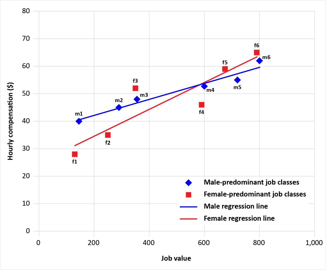
When using the equal line method, employers and pay equity committees must create two regression lines. One line represents the relationship between job values and total hourly compensation for predominantly female job classes. The other line represents the relationship between job values and total hourly compensation for predominantly male job classes.
When creating these two regression lines, there may be situations in which they cross.
Figure 1: Job values and total hourly compensation for male and female job classes, with male and female regression lines – crossed regression lines scenario
3. The rules that must be applied if the regression lines cross
In situations where the initial regression lines cross, the employer or pay equity committee must compare the compensation of predominantly male and predominantly female job classes using:
- The modified version of the equal line method set out in section 14(a) of the Pay Equity Regulations (the Regulations);
- The equal average method set out in section 49 of the Pay Equity Act (the Act);
- The segmented line method set out in section 15 of the Regulations; or,
- The sum of differences method set out in section 16 of the Regulations.ii
For information on the modified version of the equal line method, see Comparing Compensation – No. 3: What to Do When the Regression Lines Cross: The Modified version of the equal line method.
For information on the equal average method, see Comparing Compensation – No. 1: The Application of the Equal Average Method.
The method chosen by the employer or pay equity committee will depend on the organizational structure and data.
The legislation prescribes that if the regression lines cross, the employer or pay equity committee must first use the modified version of the equal line method. Should the modified version of the equal line method not work, the Act does not prescribe in which order the remaining methods should be used. Different situations will result in different decisions.
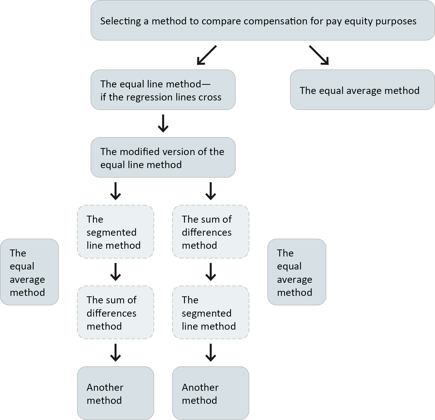
Figure 2 provides an illustration of what a decision-making process might look like:
- The equal average method is the default approach and may be implemented at any time.
- Each subsequent block is the next method to try in the event of a failure (i.e., failing to achieve pay equity).
- In some circumstances, the decision to use another method may be considered:
- If a pay equity committee determines that neither the equal average method nor the equal line method can be used to compare compensation, it may select a method that it considers appropriate.iii
- If an employer with no pay equity committee determines that neither the equal average method nor the equal line method can be used, it must apply to the Pay Equity Commissioner for authorization to use a method that it proposes.
For more information, see Comparing Compensation – No. 5: Guidance on the Use of Other Methods to Compare Compensation.
Figure 2: Selecting a method to compare compensation for pay equity purposes
4. The modified version of the equal line method
With the modified version of the equal line method, the employer or pay equity committee will apply the equal line method without taking into account the requirement that the female regression line lie entirely below the male regression line. To use this method, apply the rules set out in sections 50(1)(b) to (d) of the Pay Equity Act, without taking into account subsection 50(1)(b)(i)].
The employer will owe all female job classes below the male regression line an increase in compensation. To determine the amount of these increases, the employer or pay equity committee must use the factor prescribed in subsection 12(1) of the Pay Equity Regulations.
Once the increases are applied and the female regression line is redrawn, it is possible that the male and female regression lines will coincide. Note: The regression lines are more likely to coincide when the portion of the female regression line that was above the male regression line when they initially crossed remains relatively close to the male regression line. In this scenario, pay equity is more likely to be achieved using the modified version of the equal line method.
For more information, see Comparing Compensation – No. 3: What to Do When the Regression Lines Cross: The Modified Version of the Equal Line Method.
5. The equal average method
If the employer or pay equity committee uses the modified version of the equal line method and the regression lines remain crossed, it may choose to use the equal average method, as outlined in section 49 of the Pay Equity Act.
For more information, see Comparing Compensation – No. 1: The Application of the Equal Average Method.
6. The segmented line method
If the employer or pay equity committee uses the modified version of the equal line method and the regression lines remain crossed, it may choose to use the segmented line method, as outlined in section 15 of the Pay Equity Regulations (the Regulations).
6.1. Detailed example using the segmented line method
The following example provides step-by-step guidance on how to use the segmented line method if the regression lines remain crossed after using the modified version of the equal line method.
Company B’s pay equity plan includes six female job classes and six male job classes. Table 1 provides the total hourly compensation and job values for each of these job classes.
Table 1: Company B job classes, job values and total hourly compensation
Female job classes
| Job class | Job value | Total hourly compensation |
|---|---|---|
| f1 | 145 | $25.00 |
| f2 | 235 | $33.00 |
| f3 | 345 | $42.00 |
| f4 | 584 | $51.00 |
| f5 | 675 | $56.00 |
| f6 | 790 | $61.00 |
Male job classes
| Job class | Job value | Total hourly compensation |
|---|---|---|
| m1 | 155 | $28.00 |
| m2 | 235 | $41.00 |
| m3 | 355 | $44.00 |
| m4 | 590 | $45.00 |
| m5 | 705 | $55.00 |
| m6 | 800 | $55.00 |
6.1.1. Step 1: Create two regression lines by plotting the data on a graph
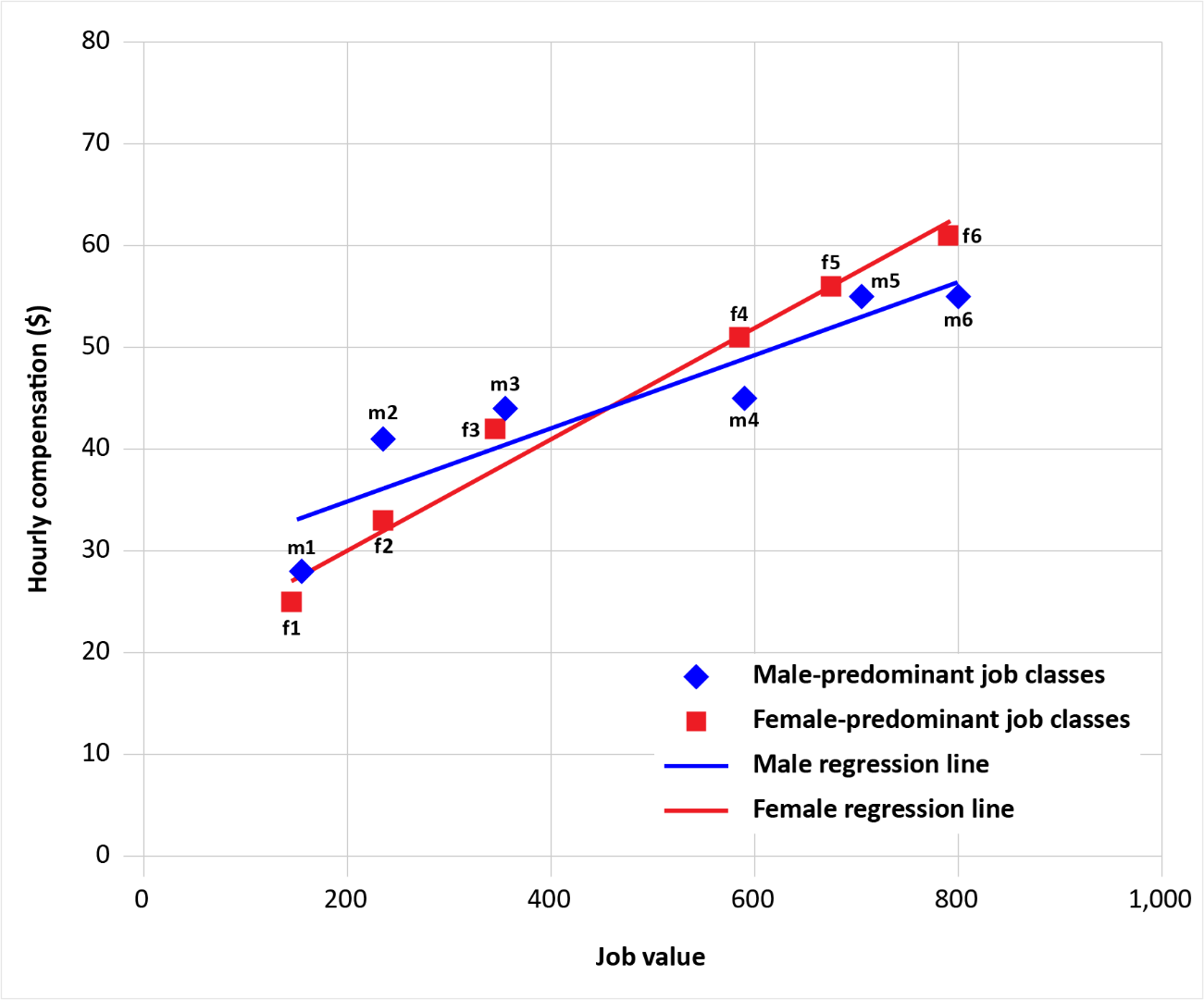
As a first step, Company B’s pay equity committee must create two regressions lines by plotting the data on a graph.
Using the data from Table 1, the pay equity committee plots total hourly compensation the y-axis and job values on the x-axis. They plot the amounts for female and male job classes separately.
Female job classes are represented by red squares, and male job classes are represented by blue diamonds.
Two regression lines are created, estimating the total hourly compensation for the male and female job classes, respectively.
After creating the two regression lines, Company B’s pay equity committee sees that the regression lines cross. The pay equity committee members proceed with the modified version of the equal line method.
After using the modified version of the equal line method, the regression lines remain crossed. Company B’s pay equity committee decides to use the segmented line method, as outlined in section 15 of the Regulations.
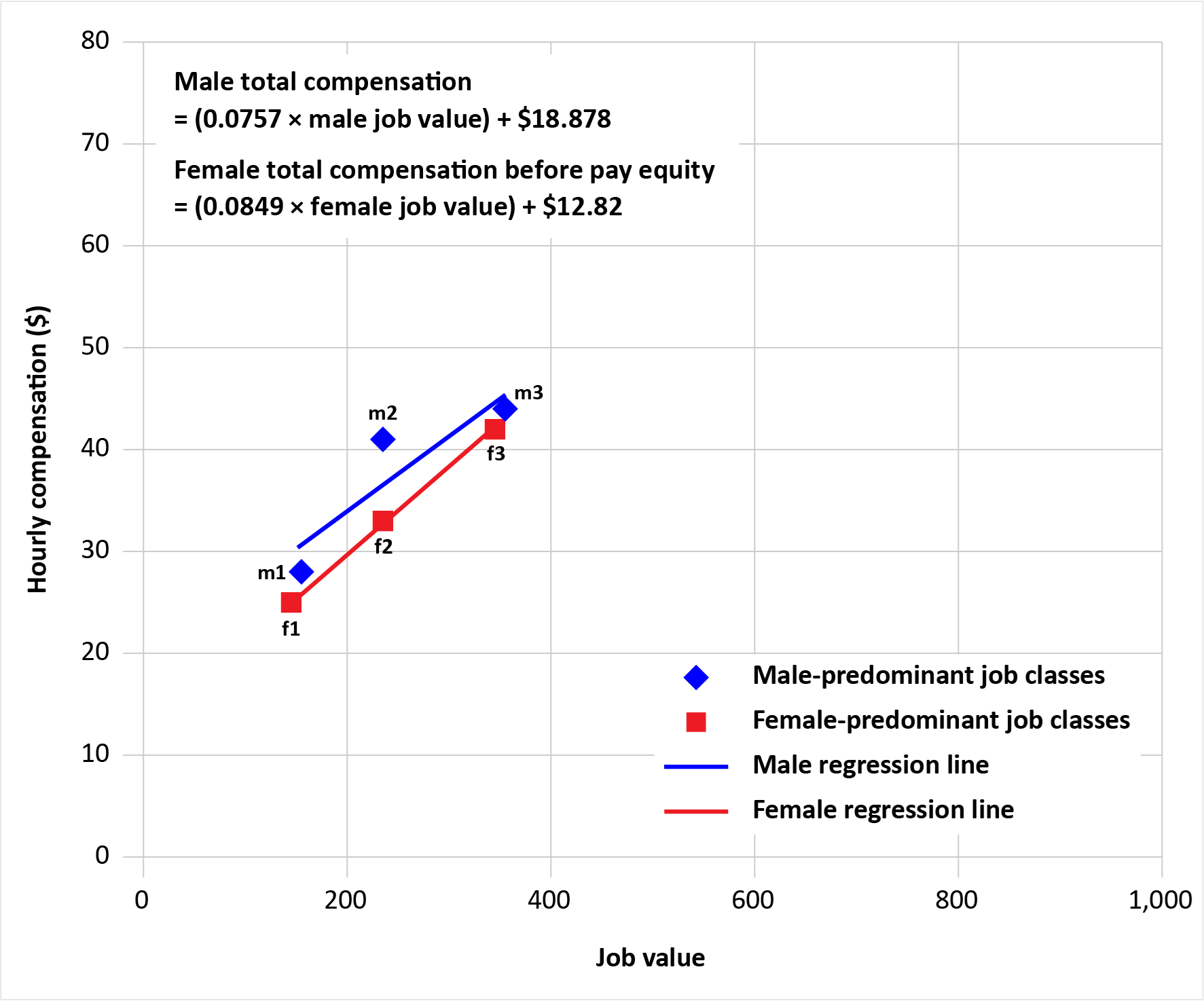
Figure 3: Job values and total hourly compensation for Company B job classes, with male and female regression lines
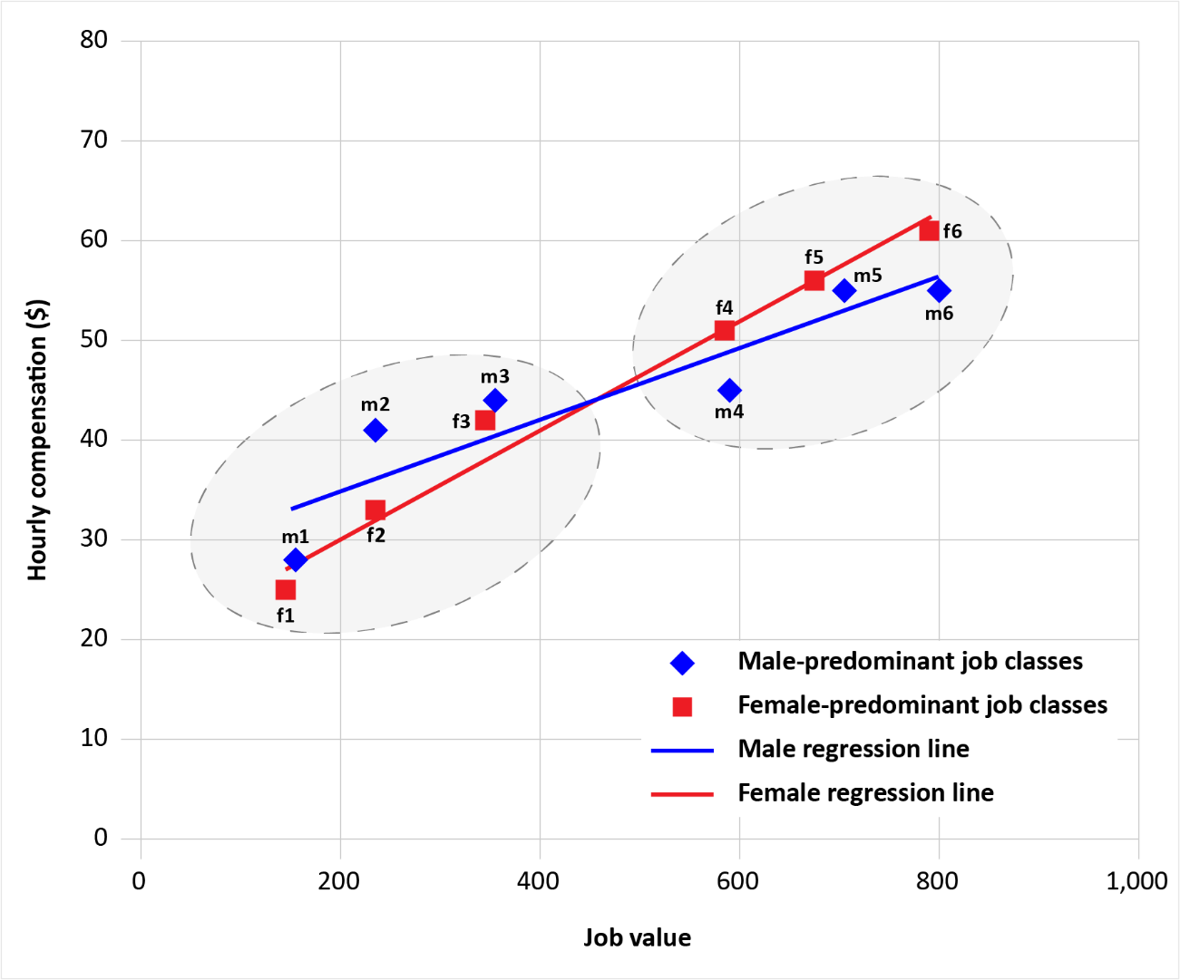
6.1.2 Step 2: Divide the job classes at the point where the male and female regression lines intersect
Following the Regulations for the segmented line method, Company B’s pay equity committee must identify the point at which the male and female regression lines cross.
Figure 4: Job values and total hourly compensation for Company B job classes, with male and female regression lines, with segments above and below the point of intersection identified
6.1.3. Step 3: Form one segment with all the job classes with job values less than the job value at which the regression lines crossiv
Next, the pay equity committee creates one segment that includes all of the job classes with job values less than the job value at which the regression lines cross.
From Figure 4, the job classes with job values less than the job value at which the regression lines cross are job classes f1, f2, f3, m1, m2 and m3.
Company B’s pay equity committee creates Table 2 to organize the data for Segment 1.
Table 2: Company B Segment 1 job classes, with job values and total hourly compensation
Female job classes
| Job class | Job value | Total hourly compensation |
|---|---|---|
| f1 | 145 | $25.00 |
| f2 | 235 | $33.00 |
| f3 | 345 | $42.00 |
Male job classes
| Job class | Job value | Total hourly compensation |
|---|---|---|
| m1 | 155 | $28.00 |
| m2 | 235 | $41.00 |
| m3 | 355 | $44.00 |
6.1.4. Step 4: Form another segment with all the job classes with job values equal to or greater than the job value at which the regression lines crossv
After identifying the job classes with job values less than the job value at the which the regression lines cross, the pay equity committee identifies the job classes with job values equal to or greater than the job value at which the regression lines cross.
From Figure 4, the job classes with job values equal to or greater than the job value at which the regression lines cross are job classes f4, f5, f6, m4, m5 and m6.
Company B’s pay equity committee creates Table 3 to organize the data for Segment 2.
Table 3: Company B Segment 2 job classes, job values and total hourly compensation
Female job classes
| Job class | Job value | Total hourly compensation |
|---|---|---|
| f4 | 584 | $51.00 |
| f5 | 675 | $56.00 |
| f6 | 790 | $61.00 |
Male job classes
| Job class | Job value | Total hourly compensation |
|---|---|---|
| m4 | 590 | $45.00 |
| m5 | 705 | $55.00 |
| m6 | 800 | $55.00 |
6.1.5. Step 5: Redraw the male and female regression lines for each segment
After creating the segments, the pay equity committee then redraws the male and female regression lines for each segment using the male and female job classes.vi Each segment must be treated as a discrete whole. Job classes in one segment must not be compared to job classes in the other segment.
If the female regression line in either segment is entirely above the male regression line in the same segment, then no pay equity gaps exist for job classes in that segment.
Company B’s pay equity committee redraws the male and female regression lines for Segment 1 using the data from Table 2.
Female job classes are represented by red squares, and male job classes are represented by blue diamonds.
The pay equity committee notes that the female regression line for Segment 1 is entirely below the male regression line.
As per the provisions in the Regulations concerning the segmented line methodvii and in the Pay Equity Act (the Act) concerning the equal line method,viii the employer owes increases in compensation to female job classes that are below the male regression line—in this case, job classes f1, f2 and f3.
Figure 5: Job values and total hourly compensation for Company B Segment 1 job classes, with male and female regression lines redrawn
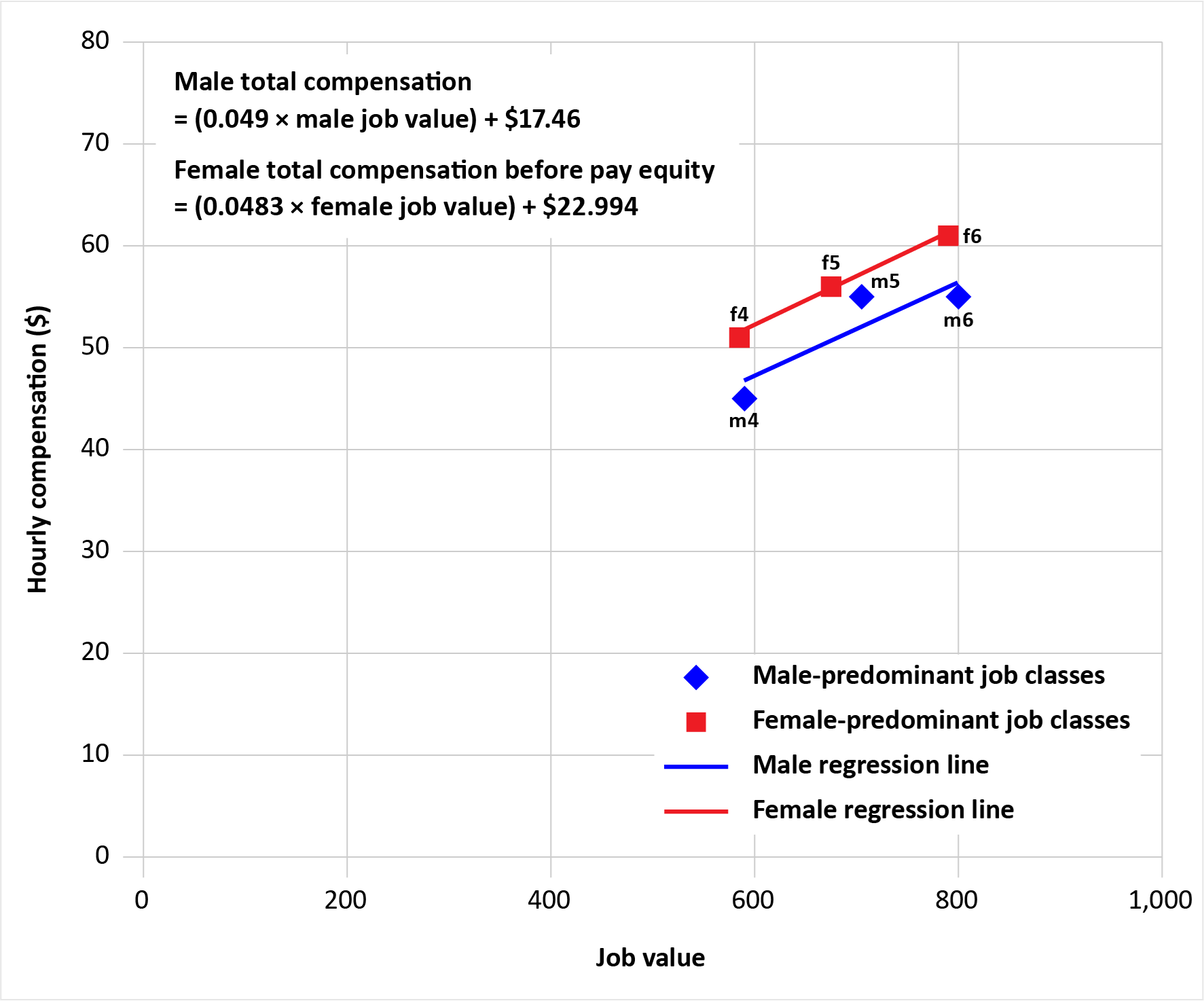
Company B’s pay equity committee then redraws the male and female regression lines for Segment 2 using the data from Table 3.
Female job classes are represented by red squares, and male job classes are represented by blue diamonds.
The pay equity committee notes that the female regression line for Segment 2 is entirely above the male regression line. Therefore, the employer does not owe increases in compensation to female job classes f4, f5 and f6.
Figure 6: Job values and total hourly compensation for Company B Segment 2 job classes, with male and female regression lines redrawn
6.1.6. Step 6: Determine the equation of the male regression line for Segment 1
Company B’s pay equity committee must now complete the comparison of total compensation exercise for female job classes in Segment 1.
To do so, Company B’s pay equity committee must determine the equation of the male regression line for the purpose of estimating total hourly compensation.
In this example, the equation of the male regression line is given by Equation 1:
Male total compensation = (0.0757 × male job value) + $18.878
Male total compensation is the total hourly compensation associated with each male job class. The slope of the Segment 1 regression line is 0.0757. Male job value is the job value associated with each male job class. The y-intercept of the Segment 1 regression line is $18.878.
Note: The equation for a regression line can be determined using graphing software such as Excel or a statistical software package such as R, SAS or SPSS. To determine the equation of the male regression line in Excel, start by right-clicking the plotted points for the male job classes and selecting “Add trend line.” Once the trend line is visible, right-click it and select “Display equation on chart.” Once the equation is displayed, it can be used to calculate the estimated compensation an employee in a male job class would be paid given different job values.
6.1.7. Step 7: Recalculate the total hourly compensation for male job classes using the equation of the male regression line and the job values of comparable female job classes
Using the data from Table 2, Company B’s pay equity committee uses the equation of the male regression line for Segment 1 to recalculate the total hourly compensation of male job classes using job values equal to those of comparable female job classes.
This step ensures that the pay equity committee is comparing female job classes with male job classes of equal value. The pay equity committee uses the equation of the male regression line to recalculate the total hourly compensation for male job classes of equal value to their female counterparts. This step is required so that female job classes can be compared to male job classes of the same job value.
Table 4 below provides the adjusted male total hourly compensation estimates for Segment 1 job classes using Equation 1, the equation of the male regression line, calculated in Step 6 above.
For example, the adjusted total hourly compensation for m1 in Table 4 is calculated as follows:
m1 adjusted total hourly compensation = (0.0757 × male job value) + $18.878
= (0.0757 × 145) + $18.878
= $29.85
The new m1 total hourly compensation amount, calculated using Equation 1, is $29.85.
For example, the adjusted total hourly compensation for m2 in Table 4 is calculated as follows:
m2 adjusted total hourly compensation = (0.0757 × male job value) + $18.878
= (0.0757 × 235) + $18.878
= $36.67
The new m2 total hourly compensation amount, calculated using Equation 1, is $36.67.
Table 4 also demonstrates that the job values of male job classes are the same as those of the female job classes.
Company B’s pay equity committee uses the new male total hourly compensation amounts for the remaining calculations to determine the increases owed to eligible female job classes in Segment 1.
The amounts in Table 2 are no longer relevant.
Table 4: Company B Segment 1 job classes, job values and total hourly compensation, with male job values equal to job values of comparable female job classes and male total hourly compensation adjusted using Equation 1
Female job classes
| Job class | Job value | Total hourly compensation |
|---|---|---|
| f1 | 145 | $25.00 |
| f2 | 235 | $33.00 |
| f3 | 345 | $42.00 |
Male job classes
| Job class | New job value* | New total hourly compensation |
|---|---|---|
| m1 | 145 | $29.85 |
| m2 | 235 | $36.67 |
| m3 | 345 | $44.99 |
|
* New male job values are equal to the job values of comparable female job classes. ** New male total hourly compensation amounts are estimated using Equation 1. |
||
6.1.8. Step 8: Calculate the factor
Now that Company B’s pay equity committee has estimated the new male total hourly compensation amounts outlined in Table 4, they must calculate the factor for each of the female job classes in Segment 1 that are owed an increase in compensation.
For this example, detailed calculations will be provided for the first female job class, f1.
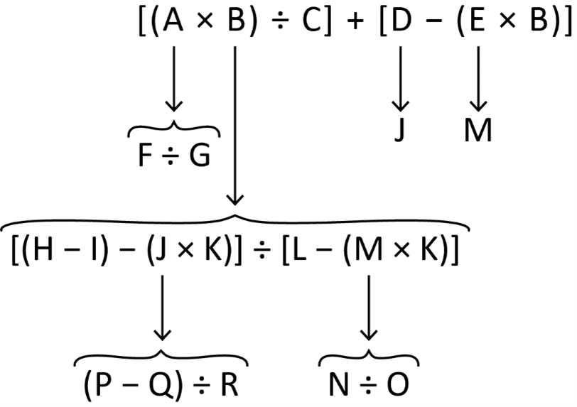
The factor is calculated using the following formula:
Factor = [(A × B) ÷ C] + [D − (E × B)]
In this formula:
A is determined by the formula A = F ÷ G, where:
F is the absolute value of the difference between the compensation associated with the predominantly female job class and the compensation associated with a predominantly male job class, were such a job class located on the male regression line, in which the value of the work performed is equal to that of the predominantly female job class.
G is the compensation associated with such a predominantly male job class.
In this example, F is the absolute value, expressed as ABS(Number), or the positive value resulting from the difference between the hourly compensation associated with the predominantly female job class and the hourly compensation associated with a predominantly male job class of equal value, were it located on the male regression line.
For female job class f1, A is calculated as follows:
A = F ÷ G
= [ABS (f1 compensation − m1 compensation)] ÷ m1 compensation
= [ABS ($25.00 − $29.85)] ÷ $29.85
= $4.85 ÷ $29.85
= 0.1626
The value to use for A in the factor calculation is 0.1626.
B is determined by the formula B = [(H − I) − (J × K)] ÷ [L − (M × K)], where:
H is the sum of the products of the job value of each predominantly female job class multiplied by the hourly compensation associated with a predominantly male job class of equal value, were it located on the male regression line.
H = (f1 job value × m1 compensation) + (f2 job value × m2 compensation)
+ (f3 job value × m3 compensation)
= (145 × $29.8545) + (235 × $36.6675) + (345 × $44.9945)
= $28,468.87
I is the sum of products of the job value for each predominantly female job class and the hourly compensation associated with that job class.
I = (f1 job value × f1 compensation) + (f2 job value × f2 compensation)
+ (f3 job value × f3 compensation)
= (145 × $25.00) + (235 × $33.00) + (345 × $42.00)
= $25,870.00
J is determined by the formula J = (P − Q) ÷ R, where:
P is the total of the compensation of all predominantly male job classes, were such job classes located on the male regression line, in which the value of the work performed is equal to that of the predominantly female job classes.
P = m1 compensation + m2 compensation + m3 compensation
= $29.8545 + $36.6675 + $44.9945
= $111.517
Q is the total of the compensation of all predominantly female job classes.
Q = f1 compensation + f2 compensation + f3 compensation
= $25.00 + $33.00 + $42.00
= $100.00
R is the sum of the absolute value of the differences, for each eligible predominantly female job class (falling below the male regression line), between the hourly compensation associated with the job class and the hourly compensation associated with a predominantly male job class of equal value, were it located on the male regression line.
R = [ABS (f1 compensation − m1 compensation)] + [ABS (f2 compensation − m2 compensation)] + [ABS (f3 compensation – m3 compensation)]
= [ABS ($25.00 − $29.8545)] + [ABS ($33.00 − $36.6675)] + [ABS ($42.00 − $44.9945)]
= $11.517
To calculate J:
J = (P − Q) ÷ R
= ($111.517 − $100.00) ÷ $11.517
= 1.0000
K is the sum of the products of the job value of each eligible predominantly female job class multiplied by the absolute value of the difference between its associated hourly compensation and the hourly compensation associated with a predominantly male job class of equal value, were it located on the male regression line.
K = [f1 job value × ABS (f1 compensation − m1 compensation)]
+ [f2 job value × ABS (f2 compensation − m2 compensation)]
+ [f4 job value × ABS (f3 compensation – m3 compensation)]
= [145 × ABS ($25.00 − $29.8545)] + [235 × ABS ($33.00 − $36.6675)]
+ [345 × ABS ($42.00 − $44.9945)]
= $2,598.8675
L is the sum of the products of the job value of each eligible predominantly female job class multiplied by the number calculated for that job class using the equation for A.
L = (f1 job value × A for f1) + (f2 job value × A for f2) + (f3 job value × A for f3)
= (145 × 0.162605) + (235 × 0.10002) + (345 × 0.066553)
= 70.0432
The calculation for A for all predominantly female job classes is determined using the formula Ai = Fi ÷ Gi, where i represents the predominantly female job class.
The calculation for A for female job class f1 is provided above.
M is determined by the formula M = N ÷ O, where:
N is the sum of the quotients calculated using the formula set out in A (i.e., A = F ÷ G) in this document, for each eligible predominantly female job class.
N = A for f1 + A for f2 + A for f3
= 0.162605 + 0.10002 + 0.66553
= 0.329178
O is the sum of the absolute values of the differences between the compensation associated with each eligible predominantly female job class and the compensation associated with a predominantly male job class of equal value, were it on the male regression line.
O = ABS (f1 compensation − m1 compensation) + ABS (f2 compensation − m2 compensation)
+ ABS (f3 compensation – m3 compensation)
= ABS ($25.00 − $29.8545) + ABS ($33.00 − $36.6675)
+ ABS ($42.00 − $44.9945)
= $11.517
To calculate M:
M = N ÷ O = 0.329178 ÷ 11.517 = 0.02858
Therefore, to calculate B:
B = [(H − I) − (J × K)] ÷ [L − (M × K)]
= [($28,468.87 − $25,870.00) − (1.0000 × $2,598.8675)]
÷ [(70.0432 − (0.02858 × $2,598.8675)]
= ($2,598.87 − $2,598.87) ÷ [(70.0432 − 74.2756]
= 0.0000
The value to use for B in the factor calculation is 0.0000
C is calculated as follows:
C is the absolute value of the difference between the hourly compensation associated with the predominantly female job class and the hourly compensation associated with a predominantly male job class of equal value, were it on the male regression line.
C = ABS (f1 compensation − m1 compensation)
= ABS ($25.00 − $29.8545)
= $4.8545
The value to use for C in the factor calculation is 4.8545.
D is calculated as follows:
D is the same value calculated for J.
D = J = 1.0000
The value to use for D in the factor calculation is 1.0000.
E is calculated as follows:
E is the same value calculated for M.
E = M = 0.02858
The value to use for E in the factor calculation is 0.02858.
The final calculation of the factor for female job class f1 is as follows:
Factor = [(A × B) ÷ C] + [(D − (E × B)
= [(0.162605 × 0.000) ÷ 4.8545] + [(1.000 − (0.02858 × 0.0000)
= 1.0000
The final factor calculation amount is 1.0000.
6.1.9. Step 9: Determine the increase in compensation
Company B’s pay equity committee calculates that the factor for female job class f1 is 1.0000.
Increases in compensations for eligible female job classes are calculated by multiplying the difference between the hourly compensation of a female job class and the hourly compensation associated with a male job class of same value by the factor associated with that female job class.
The increase in compensation for an eligible female job class is calculated using the following formula:
Increase in compensation = C × factor
For female job class f1, the increase in compensation is calculated as follows:
Increase in compensation = C for f1 × factor for f1
= $4.8545 × 1.0000
= $4.8545
The increase in total hourly compensation for female job class f1 is $4.8545.
The total hourly compensation after pay equity for female job class f1 then becomes $25.00 + $4.8545 = $29.85.
Increases in compensation for all female job classes in Segment 1 that were calculated by Company B’s pay equity committee are provided in Table 5.
Table 5: Increases in compensation after pay equity
| Female job class | Total hourly compensation before pay equity | A × B ÷ C | D − (E × B) | C | Factor | Increase in total hourly compensation (C × factor) | Total hourly compensation after pay equity |
|---|---|---|---|---|---|---|---|
| f1 | $25.00 | 0.0000 | 1.0000 | $4.85 | 1.0000 | $4.85 | $29.85 |
| f2 | $33.00 | 0.0000 | 1.0000 | $3.67 | 1.0000 | $3.67 | $36.67 |
| f3 | $42.00 | 0.0000 | 1.0000 | $2.99 | 1.0000 | $2.99 | $44.99 |
6.1.10. Step 10: Graph male and female job class data after pay equity adjustment
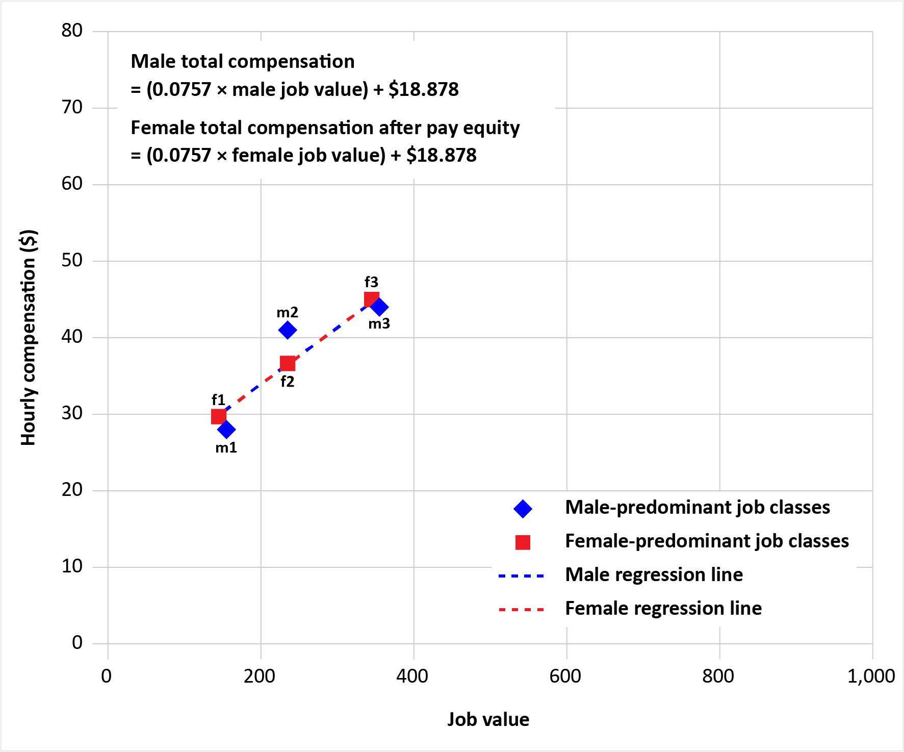
As a final step, Company B’s pay equity committee must create a new graph for Segment 1 to verify that the increases in compensation associated with eligible female job classes have been calculated in such a way that, after the increases, the female regression line coincides with the male regression line.ix
The pay equity committee graphs the new total compensation for female job classes after pay equity using the data from Table 5 and the total compensation amounts for male job classes using the data from Table 2.
Figure 7 shows the new graph. The female and male regression lines now coincide.
Figure 7: Job values and total hourly compensation for Company B Segment 1 job classes after pay equity adjustment
If using the segmented line method does not make the male and female regression lines coincide without reducing the compensation of any job class, the employer or pay equity committee must use the equal average method outlined in section 49 of the Act or the sum of differences method set out in section 16 of the Regulations to compare compensation.x
7. The sum of differences method
If the regression lines remain crossed after using the modified version of the equal line method, employers and pay equity committees may choose to use the sum of differences method to determine the compensation increases owed.xi
Under this approach, the male regression line is used to plot the female job classes. For every female job class, the employer or pay equity committee will need to determine the compensation a male job class of equal job value would receive if it were plotted on the male regression line. The difference is then calculated between the total compensation of each female job class and the corresponding male job class.
To determine the increase owed to each female job class below the male regression line, this difference is then multiplied by a factor described in section 16(2) of the Pay Equity Regulations (the Regulations).
7.1. Detailed example using the sum of differences method
The following example provides step-by-step guidance on how to use the sum of differences method if the regression lines remain crossed after using the modified version of the equal line method.
For this example, Company B’s pay equity committee has calculated the total compensation for each female and male job class. To compare total compensation, the pay equity committee decides to use the equal line method.
When making the graph, Company B’s pay equity committee sees that the regression lines cross.
Therefore, the committee follows the Pay Equity Act (the Act) and uses the modified version of the equal line method outlined in section 14(a) of the Regulations.
Company B’s pay equity plan includes seven female job classes and six male job classes. Table 6 provides the total hourly compensation and job value for each of these job classes.
Table 6: Company B job classes, job values and total hourly compensation
Female job classes
| Job class | Job value | Total hourly compensation |
|---|---|---|
| f1 | 190 | $25.00 |
| f2 | 300 | $42.00 |
| f3 | 550 | $45.00 |
| f4 | 594 | $44.00 |
| f5 | 675 | $60.00 |
| f6 | 765 | $50.00 |
| f7 | 792 | $70.00 |
Male job classes
| Job class | Job value | Total hourly compensation |
|---|---|---|
| m1 | 200 | $35.00 |
| m2 | 250 | $40.00 |
| m3 | 550 | $48.00 |
| m4 | 599 | $50.00 |
| m5 | 720 | $55.00 |
| m6 | 810 | $60.00 |
| m7 | n/a | n/a |
7.1.1. Step 1: Create two regression lines by plotting the data on a graph
As a first step, Company B’s pay equity committee must create two regression lines by plotting the data on a graph.
Using the data from Table 6, the pay equity committee plots total hourly compensation on the y-axis and job values on the x-axis. They plot the amounts for the female and male job classes separately.
Female job classes are represented by red squares, and male job classes are represented by blue diamonds.
Two regression lines are created, estimating the total hourly compensation for male and female job classes, respectively.
Figure 8: Company B job classes, job values and total hourly compensation, with male and female regression lines
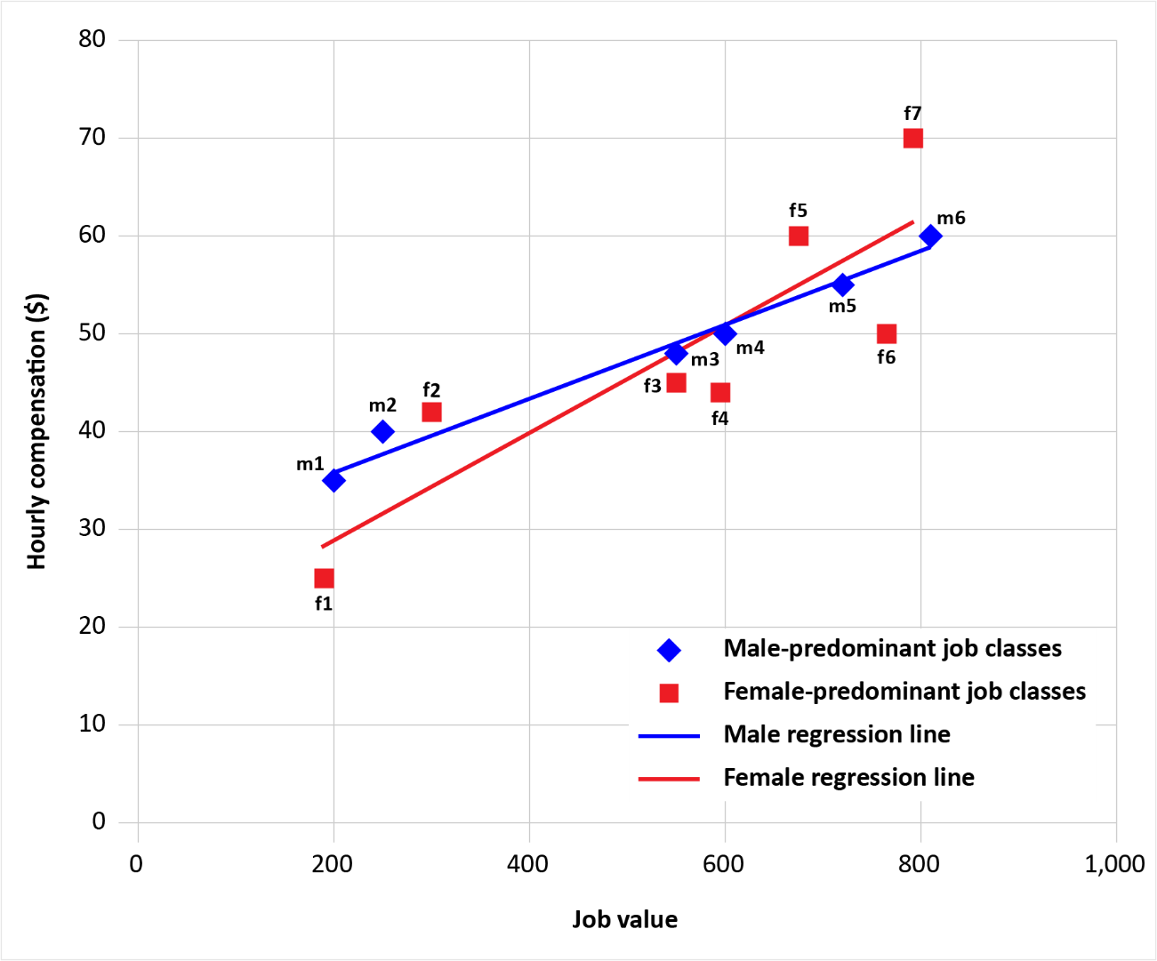
7.1.2. Step 2: Identify female job classes falling below the male regression line
Following the provisions in the Act for the equal line methodology, all female job classes below the male regression line are eligible for a pay increase.
After Company B’s pay equity committee creates the regression lines, it identifies the female job classes that are below the male regression line. These are the female job classes that are eligible for a pay increase.
From Figure 8, female job classes f1, f3, f4, and f6 all fall below the male regression line and are eligible for a pay increase.
7.1.3. Step 3: Determine the equation of the male regression line
Some female job classes in Company B’s pay equity plan are owed an increase in compensation. The increase in compensation for each of these job classes must be determined by multiplying the factor by the difference between the compensation associated with the female job class and the compensation associated with a male job class with an equal job value, were such a job class located on the male regression line.xii
To begin, Company B’s pay equity committee must calculate the difference between the compensation associated with each female job class and the compensation associated with a male job class with an equal job value, were such a job class located on the male regression line. To do this, the pay equity committee must determine the equation of the male regression line for the purpose of estimating total hourly compensation.
In this example, the equation of the male regression line is given by Equation 1:
Male total compensation = (0.0371 × male job value) + $28.676
Male total compensation is the total hourly compensation associated with each male job class. The slope of the regression line is 0.0371. Male job value is the job value associated with each male job class. The y-intercept of the regression line is $28.676.
Note: The equation for a regression line can be determined using graphing software such as Excel or a statistical software package such as R, SAS or SPSS. To determine the equation of the male regression line in Excel, start by right-clicking the plotted points for the male job classes and selecting “Add trend line.” Once the trend line is visible, right-click it and select “Display equation on chart.” Once the equation is displayed, it can be used to calculate the estimated compensation an employee in a male job class would be paid given different job values.
Figure 9: Company B job classes, job values and total hourly compensation, with the male regression line plotted and its equation displayed
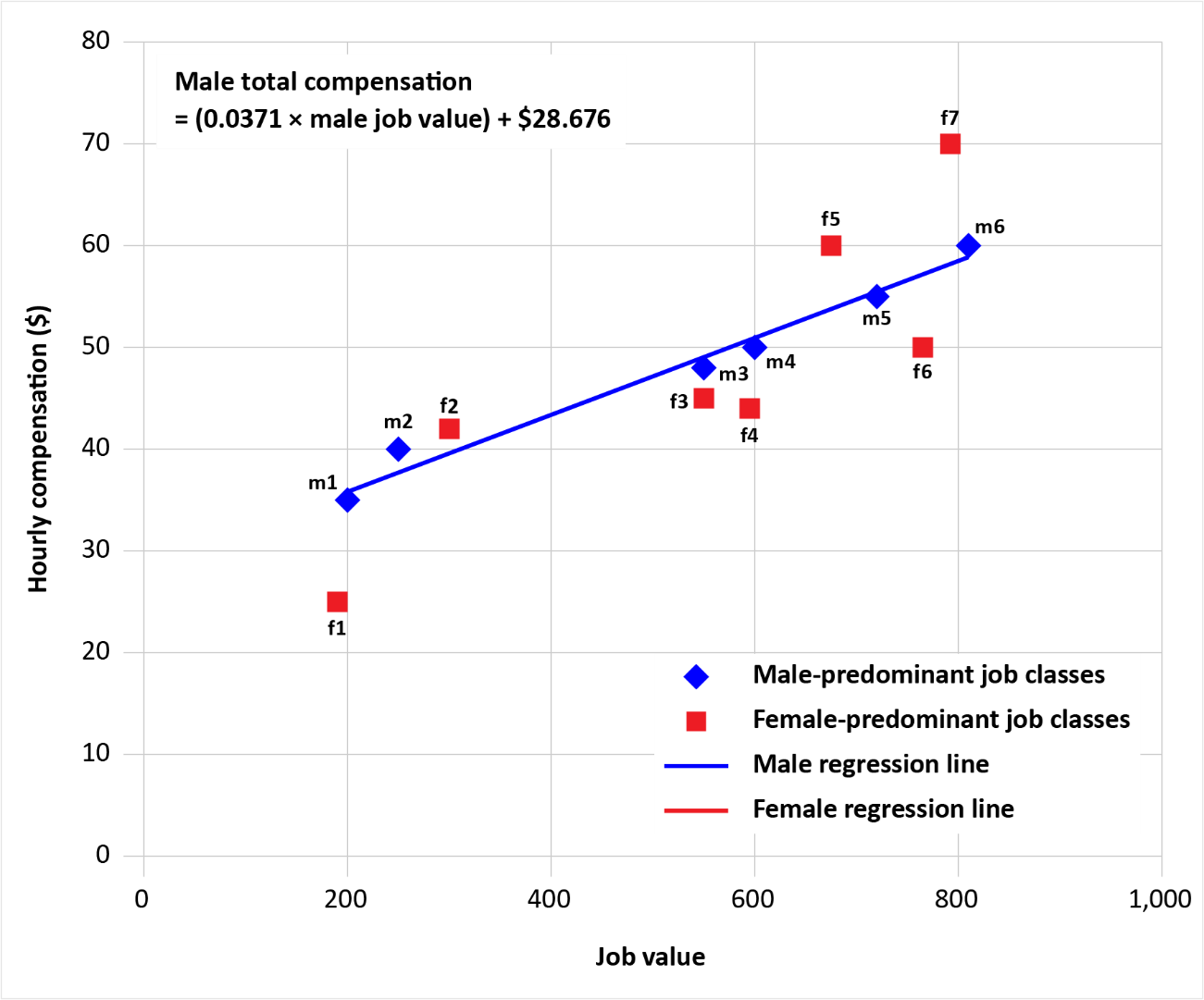
The blue regression line in Figure 9 represents the estimated male compensation based on the male job values. Its formula is given by Equation 1:
Male total compensation = (slope × male job value) + y-intercept
Male total compensation = (0.0371 × male job value) + $28.676
7.1.4. Step 4: Recalculate total hourly compensation for male job classes using the equation of the male regression line and the job values of comparable female job classes
Using the data from Table 6, Company B’s pay equity committee uses the equation of the male regression line to recalculate the total hourly compensation of male job classes using job values equal to those of comparable female job classes.
This step ensures that the pay equity committee is comparing female job classes with male job classes of equal value. The pay equity committee uses the equation of the male regression line to recalculate the total hourly compensation for male job classes of equal value to their female counterparts. This step is required so that female job classes can be compared to male job classes of the same job value.
Table 7 below provides the adjusted male total hourly compensation estimates using Equation 1, the equation of the male regression line, calculated in Step 3 above.
For example, the adjusted total hourly compensation for m1 in Table 7 is calculated as follows:
m1 adjusted total hourly compensation = (0.0371 × male job value) + $28.676
= (0.0371 × 190) + $28.676
$35.73
The new m1 total hourly compensation, calculated using Equation 1, is $35.73.
For example, the adjusted total hourly compensation for m2 in Table 7 is calculated as follows:
m2 adjusted total hourly compensation = (0.0371 × male job value) + $28.676
= (0.0371 × 300) + $28.676
= $39.806
The new m2 total hourly compensation, calculated using Equation 1, is $39.81.
Company B’s pay equity committee uses the new male total hourly compensation for the factor calculations to determine the increases owed to eligible female job classes. The amounts in Table 6 are no longer relevant.
Table 7: Company B job classes, job values and total hourly compensation, with male job values equal to job values of comparable female job classes and male total hourly compensation adjusted using Equation 1
Female job classes
| Job class | Job value | Total hourly compensation |
|---|---|---|
| f1 | 190 | $25.00 |
| f2 | 300 | $42.00 |
| f3 | 550 | $45.00 |
| f4 | 594 | $44.00 |
| f5 | 675 | $60.00 |
| f6 | 765 | $50.00 |
| f7 | 792 | $70.00 |
Male job classes
| Job class | New job value* | New total hourly compensation** |
|---|---|---|
| m1 | 190 | $35.73 |
| m2 | 300 | $39.81 |
| m3 | 550 | $49.08 |
| m4 | 594 | $50.71 |
| m5 | 675 | $53.72 |
| m6 | 765 | $57.06 |
| m7 | 792 | $58.06 |
|
* New male job values are equal to the job values of comparable female job classes. ** New male total hourly compensation amounts are estimated using Equation 1. |
||
7.1.5. Step 5: Calculate the factor
To calculate the factor, use the formula Factor = (A − B) ÷ C, where:
A is the sum of the compensation associated with predominantly male job classes, were such job classes located on the male regression line, in which the value of the work performed is equal to that of the predominantly female job classes.
Example calculation for A:
A = m1 compensation + m2 compensation + m3 compensation + m4 compensation
+ m5 compensation + m6 compensation + m7 compensation
= $35.73 + $39.81 + $49.08 + $50.71 + $53.72 + $57.06 + $58.06
= $344.16
The value to use for A in the factor calculation is $344.16.
B is the sum of the compensation associated with the predominantly female job classes or the value determined for A, whichever is less.
Example calculation for B:
B = f1 compensation + f2 compensation + f3 compensation + f4 compensation
+ f5 compensation + f6 compensation + f7 compensation
= $25.00 + $42.00 + $45.00 + $44.00 + $60.00 + $50.00 + $70.00
= $336.00
The value to use for B in the factor calculation is $336.00.
C is the sum of the absolute values of the differences, for each predominantly female job class that is located below the male regression line, between the compensation associated with the job class and the compensation associated with a predominantly male job class, were such a job class located on the male regression line, in which the value of the work performed is equal to that of the predominantly female job class.xiii
Example calculation for C:
C = ABS (f1 compensation − m1 compensation) + ABS (f3 compensation – m3 compensation)
+ ABS (f4 compensation – m4 compensation) + ABS (f6 compensation – m6 compensation)
= ABS ($25.00 − $35.73) + ABS ($45.00 − $49.08)
+ ABS ($44.00 − $50.71) + ABS ($50.00 − $57.06)
= $10.73 + $4.08 + $6.71 + $7.06
= $28.58
The value to use for C in the factor calculation is $28.58.
Therefore, to calculate the factor:
Factor = (A − B) ÷ C
= ($344.16 – $336.00) ÷ $28.58
= 0.2856
The value of the factor in this example is 0.2856.
7.1.6. Step 6: Determine the increase in compensation using the value calculated for the factor
Once the factor is calculated, use this value to determine the increase in compensation for each female job class below the male regression line.
In this example, the female job classes below the male regression are job classes f1, f3, f4 and f6.
To begin, Company B’s pay equity committee determines the absolute value (ABS) of the difference between the compensation of each female job class owed an increase in compensation and the estimated compensation of each corresponding male job class with the same job value.xiv That is, the compensation of each eligible female job class is subtracted from the estimated compensation of a male job class with the same job value, calculated using the equation of the male regression line.
For job class f1:
Difference in compensation = ABS (f1 compensation − m1 compensation)
= ABS ($25.00 − $35.73)
= $10.73
For job class f3:
Difference in compensation = ABS (f3 compensation – m3 compensation)
= ABS ($45.00 − $49.08)
= $4.08
For job class f4:
Difference in compensation = ABS (f4 compensation – m4 compensation)
= ABS ($44.00 − $50.71)
= $6.71
For job class f6:
Difference in compensation = ABS (f6 compensation – m6 compensation)
= ABS ($50.00 − $57.06)
= $7.06
For job class f1, this difference is $10.73.
For job class f3, this difference is $4.08.
For job class f4, this difference is $6.71.
For job class f6, this difference is $7.06.
The pay equity committee then multiplies each of these differences by the factor to calculate the increase in compensation owed to each female job class requiring an adjustment.xv
For job class f1:
Increase in compensation = ABS (f1 compensation − m1 compensation) × factor
= $10.73 × 0.2856
= $3.06
For job class f3:
Increase in compensation = ABS (f3 compensation – m3 compensation) × factor
= $4.08 × 0.2856
= $1.17
For job class f4:
Increase in compensation = ABS (f4 compensation – m4 compensation) × factor
= $6.71 × 0.2856
= $1.92
For job class f6:
Increase in compensation = ABS (f6 compensation – m6 compensation) × factor
= $7.06 × 0.2856
= $2.01
For job class f1, the pay increase is $3.06.
For job class f3, the pay increase is $1.17.
For job class f4, the pay increase is $1.92.
For job class f6, the pay increase is $2.01.
7.1.7. Step 7: Determine the new hourly compensation for each predominant female job class requiring an adjustment
To determine the new total hourly compensation rates, the pay increases calculated in step 6 above are added to the total hourly compensation of each female job class requiring an adjustment (from Table 6):
- The adjusted compensation for job class f1 is $25.00 + $3.06 = $28.06.
- The adjusted compensation for job class f3 is $45.00 + $1.17 = $46.17.
- The adjusted compensation for job class f4 is $44.00 + $1.92 = $45.92.
- The adjusted compensation for job class f6 is $50.00 + $2.01 = $52.01.
7.1.8. Step 8: Verify total amounts
To determine if the sum of differences method was successful, Company B’s pay equity committee needs to ensure that the following totals are equal after all required adjustments are made:
Total 1 is the sum of the absolute values (ABS) of the differences between the adjusted compensation paid to female job classes below the male regression line and the compensation that would be paid to male job classes with the same job values if they were on the male regression line.
Total 1 = ABS (f1 adjusted compensation − m1 compensation)
+ ABS (f3 adjusted compensation – m3 compensation)
+ ABS (f4 adjusted compensation – m4 compensation)
+ ABS (f6 compensation – m6 compensation)
= ABS ($28.06 − $35.73) + ABS ($46.17 − $49.08)
+ ABS ($45.92 − $50.71) + ABS ($52.01 − $57.06)
= $20.42
The amount for Total 1 is $20.42.
Total 2 is the sum of the absolute values (ABS) of the differences between the compensation paid to female job classes above the male regression line and the compensation that would be paid to male job classes with the same job values if they were on the male regression line.
Total 2 = ABS (f2 compensation – m2 compensation)
+ ABS (f5 compensation – m5 compensation)
+ ABS (f7 compensation – m7 compensation)
= ABS ($42.00 − $39.81) + ABS ($60.00 − $53.72) + ABS ($70.00 − $58.06)
= $20.42
The amount for Total 2 is $20.42.
Since Total 1 = Total 2, the condition for pay equity under the sum of differences method has been satisfied.
If the amounts were not equal, the pay equity committee would have to use the equal average method to compare the total compensation of female and male job classes.
8. Referenced Pay Equity Act provisions
Group of Employers
4 (1) Two or more employers described in any of paragraphs 3(2)(e) to (i) that are subject to this Act may form a group and apply to the Pay Equity Commissioner to have the group of employers recognized as a single employer.
Comparison
47 An employer — or, if a pay equity committee has been established, that committee — that has calculated under section 44 the compensation associated with each job class must, using the compensation so calculated, compare, in accordance with sections 48 to 50, the compensation associated with the predominantly female job classes with the compensation associated with the predominantly male job classes, for the purpose of determining whether there is any difference in compensation between those job classes.
Compensation comparison methods
48 (1) The comparison of compensation must be made in accordance with the equal average method set out in section 49 or the equal line method set out in section 50.
Other methods
(2) Despite subsection (1),
(a) if an employer determines that neither of the methods referred to in that subsection can be used, the employer must
(i) apply to the Pay Equity Commissioner for authorization to use a method for the comparison of compensation that is prescribed by regulation or, if the regulations do not prescribe a method or the employer is of the opinion that the prescribed method cannot be used, a method that it proposes, and
(ii) use the method for the comparison of compensation that the Pay Equity Commissioner authorizes; and
(b) if a pay equity committee determines that neither of the methods referred to in that subsection can be used, the committee must use a method for the comparison of compensation that is prescribed by regulation or, if the regulations do not prescribe a method or the committee is of the opinion that the prescribed method cannot be used, a method that it considers appropriate.
Equal average method
49 (1) An employer or pay equity committee, as the case may be, that uses the equal average method of comparison of compensation must apply the following rules:
(a) the average compensation associated with the predominantly female job classes within a band — or, if there is only one such job class within a band, the compensation associated with that job class — is to be compared to
(i) if there is more than one predominantly male job class within the band, the average compensation associated with the predominantly male job classes within the band,
(ii) if there is only one predominantly male job class within the band, the compensation associated with that job class, or
(iii) if there are no predominantly male job classes within the band, the compensation calculated under paragraph (b);
(b) the compensation for the purpose of subparagraph (a)(iii) is the following:
(i) the amount determined by the formula
(A × B)/C
where
A
is the average compensation associated with the predominantly male job classes — or if there is only one such job class, the compensation associated with that job class — that are within the band that is closest to the band within which the predominantly female job class or classes are located,
B
is the average value of the work performed in the predominantly female job classes within the band or, if there is only one such job class, the value of the work performed in that job class, and
C
is the average value of the work performed in the predominantly male job classes within the band referred to in the description of A or, if there is only one such job class, the value of the work performed in that job class, or
(ii) despite subparagraph (i), if there is at least one predominantly male job class within each of two bands that are equidistant from the band within which the predominantly female job class or classes are located, and there is no other band containing at least one predominantly male job class that is closer to that band, the amount determined by the formula
(A + B)/2
where
A
is the average compensation associated with the predominantly male job classes within one of the two bands or, if there is only one such job class, the compensation associated with that job class, and
B
is the average compensation associated with the predominantly male job classes within the other band or, if there is only one such job class, the compensation associated with that job class;
(c) the compensation associated with a predominantly female job class within a band is to be increased only if
(i) that compensation is lower than the compensation or average compensation referred to subparagraph (a)(i), (ii) or (iii), as the case may be, and
(ii) the average compensation associated with the predominantly female job classes within the band — or, if there is only one such job class, the compensation associated with that job class — is lower than the compensation or average compensation referred to subparagraph (a)(i), (ii) or (iii), as the case may be;
(d) if the compensation associated with a predominantly female job class within a band is to be increased, the increase is to be determined by multiplying the factor calculated in accordance with the regulations by an amount equal to the difference between the compensation associated with the job class and the compensation or average compensation referred to subparagraph (a)(i), (ii) or (iii), as the case may be; and
(e) an increase in compensation associated with the predominantly female job class or classes within a band is to be made in such a way that, after the increase, the average compensation associated with the predominantly female job classes within the band — or, if there is only one such job class, the compensation associated with that job class — is equal to the compensation or average compensation referred to subparagraph (a)(i), (ii) or (iii), as the case may be.
Definition of band
(2) In this section, band means a range, as determined by an employer or pay equity committee, as the case may be, of values of work that the employer or committee considers comparable.
Equal line method
50 (1) An employer or pay equity committee, as the case may be, that uses the equal line method of comparison of compensation must apply the following rules:
(a) a female regression line must be established for the predominantly female job classes and a male regression line must be established for the predominantly male job classes;
(b) the compensation associated with a predominantly female job class is to be increased only if
(i) the female regression line is entirely below the male regression line, and
(ii) the predominantly female job class is located below the male regression line;
(c) if the compensation associated with a predominantly female job class is to be increased, the increase is to be determined by multiplying the factor calculated in accordance with the regulations by an amount equal to the difference between the compensation associated with the predominantly female job class and the compensation associated with a predominantly male job class, were such a job class located on the male regression line, in which the value of the work performed is equal to that of the predominantly female job class; and
(d) an increase in compensation associated with the predominantly female job classes is to be made in such a way that, after the increase, the female regression line coincides with the male regression line.
Crossed regression lines
(2) Despite paragraphs (1)(b) to (d), if the female regression line crosses the male regression line, an employer or pay equity committee, as the case may be, must apply the rules for the comparison of compensation that are prescribed by regulation.
Referenced Pay Equity Regulations
Rules if Regression Lines Cross
Choice of method
14 For the purposes of subsection 50(2) of the Act, the following rules apply:
(a) an employer — or, if a pay equity committee has been established, that committee — must apply the rules set out in paragraphs 50(1)(b) to (d) of the Act, without taking into account subparagraph 50(1)(b)(i); and
(b) if the application of the rules in paragraph (a) does not cause the regression lines to coincide without reducing the compensation associated with any job class, the employer or pay equity committee, as the case may be, must instead compare the compensation using
(i) the equal average method set out in section 49 of the Act,
(ii) the segmented line method set out in section 15, or
(iii) the sum of differences method set out in section 16.
Segmented line method
15 An employer or pay equity committee, as the case may be, that uses the segmented line method must apply the following rules:
(a) the employer or pay equity committee must divide the predominantly female job classes and the predominantly male job classes into the following two segments:
(i) one segment that includes the job classes in which the value of work performed is less than the value at which the regression lines established under paragraph 50(1)(a) of the Act intersect, and
(ii) one segment that includes the job classes in which the value of work performed is equal to or greater than the value at which the regression lines established under that paragraph intersect;
(b) for each segment, the employer or pay equity committee must establish a female regression line for the predominantly female job classes in the segment and a male regression line for the predominantly male job classes in the segment;
(c) in a segment in which the female regression line is entirely below the male regression line, the employer or pay equity committee must apply the rules set out in paragraphs 50(1)(b) to (d) of the Act, and if the application of those rules does not cause the male and female regression lines to coincide without reducing the compensation associated with any job class, the employer or committee must use the equal average method set out in section 49 of the Act or the sum of differences method set out in section 16 to compare the compensation associated with all predominantly female job classes and predominantly male job classes; and
(d) in a segment in which the female regression line crosses the male regression line, the employer or committee must apply the rules set out in paragraphs 50(1)(b) to (d) of the Act, without taking into account subparagraph 50(1)(b)(i), and if the application of those rules does not cause the male and female regression lines to coincide without reducing the compensation associated with any job class, the employer or committee must use the equal average method set out in section 49 of the Act or the sum of differences method set out in section 16 to compare the compensation associated with all predominantly female job classes and predominantly male job classes.
Sum of differences method
16 (1) The employer or pay equity committee, as the case may be, that uses the sum of differences method must multiply, for each predominantly female job class that is located below the male regression line established under paragraph 50(1)(a) of the Act, the factor calculated in accordance with subsection (2) by the absolute value of the difference between the compensation associated with the predominantly female job class and the compensation associated with a predominantly male job class, were such a job class located on the male regression line, in which the value of the work performed is equal to that of the predominantly female job class.
Factor
(2) For the purposes of subsection (1), the factor is the result of the formula
(A − B) ÷ C
where
A is the sum of the compensation associated with predominantly male job classes, were such job classes located on the male regression line, in which the value of the work performed is equal to that of the predominantly female job classes;
B is the sum of the compensation associated with the predominantly female job classes or the value determined for A, whichever is less; and
C is the sum of the absolute values of the differences, for each predominantly female job class that is located below the male regression line, between the compensation associated with the job class and the compensation associated with a predominantly male job class, were such a job class located on the male regression line, in which the value of the work performed is equal to that of the predominantly female job class.
Increase in compensation
(3) The increase in compensation associated with a predominantly female job class located below the male regression line is the product calculated in accordance with subsection (1) in respect of that job class.
Clarification
17 The segmented line method set out in section 15 and the sum of differences method set out in section 16 are to be applied without regard either to the number of employees or to the number of positions in a job class.